Fouling mechanism and screening of backwash parameters: Seawater ultrafiltration case
Article information
Abstract
This work deals with the membrane fouling mode and the unclogging in seawater ultrafiltration process. The identification of the fouling mechanism by modeling the experimental flux decline was performed using both the classical models of Hermia and the combined models of Bolton. The results show that Bolton models did not bring more precise information than the Hermia’s and the flux decline can be described by one of the four Hermia’s models since the backwash interval is ≤ 60 min. An experimental screening study has been then conducted to choose among 5 parameters (backwash interval, duration, pulses and the flow-rate or injected hypochlorite concentration) those that are the most influential on the fouling and the net water production. It has emerged that fouling is mainly affected by the backwash interval; its prolongation from 30 to 60 min engenders an increase in the reversible fouling and a decrease in the irreversible fouling. This later is also significantly reduced when the hypochlorite concentration increases from 4.5 to 10 ppm. Moreover, the net water production significantly increases with increasing the filtration duration up to 60 min and decreases with decreasing the backwash duration and backwash flow-rate from 10 to 40 s and from 15 to ≥ 20 L.min−1, respectively.
1. Introduction
Ultrafiltration (UF) is an excellent alternative to the conventional pretreatment of the seawater reverse osmosis process as it delivers a high and constant produced water quality. UF allows the removal of the major contaminants present in seawater (natural organic matter, bacteria and viruses). Those contaminants contribute to the fouling of membranes which decreases the water productivity and increases the operational cost [1]. A physical backwash is periodically applied to remove the deposited material on and/or in the membrane and restore the operation productivity. A chemical cleaning is sometimes applied to irreversible foulants that haven’t been removed during physical cleaning [1]. It is important to identify the fouling mechanism and to select the optimal operating conditions of “filtration/cleaning” in order to optimize the membrane unclogging.
Identifying the fouling mechanism would guide the choice of the membrane cleaning strategy [2–4]. It relies on the flux decline modeling using different mathematical models. The most used models are the individual models of Hermia [5] which describe the fouling as: cake formation, intermediate blocking, pore constriction, and complete blocking. These models were originally developed for frontal filtration at constant pressure [6–9]. However, it has been demonstrated that, under specific conditions, Hermia models could be applied in tangential filtration [10–21]. Hong et al. [22] showed during tangential filtration of colloidal suspensions that the filtration process before the “pseudo stationary state” is similar to the frontal filtration. Moreover, the transverse flow velocity, under laminar flow conditions, has no effect on the permeate flow; its effect is observed only when a steady state permeate flow is reached. Redkar et al. [23] and Romero et al. [24] also showed that the particles accumulation rate on the membrane surface and flux reduction rate do not depend on the shear rate, and follow the frontal filtration laws until the stationary state. This implies that in the early stages of the tangential filtration, most of the particles reaching the membrane surface by the permeate flux are deposited in the cake layer and, the longitudinal transport of the excess particles by transverse flow is negligible. Thus, Razi et al. [13] found from Hermia models that cake formation was the dominant mechanism during cross flow microfiltration of tomato juice at Reynolds ≤ 750 and transmembrane pressure (TMP) range of 1–3 bar. In addition, according to Li et al. [17], at 0.7 m.s−1 tangential velocity and 1bar TMP, the pore constriction model could describe the flux decrease during raw rice wine tangential microfiltration. As the velocity increases to 1 m.s−1, both models (cake formation and pore constriction) could predict fouling behavior with alternative dominance between the two as pressure increases from 1 to 2 bar.
In some cases, the individual Hermia models could not describe the fouling behavior during the filtration probably because of a combination of different fouling mechanisms. Ho and Zidney [25] developed the first combined model to describe clogging behavior during constant pressure proteins microfiltration. The model describes the transition from initial clogging by pore blockage followed by deposit formation on the blocked surface areas. This model was used as alternative to Hermia models in the case of whey wastewater tangential UF at TMP of 3 and 5 bar and concentration range of [0.5–8 g/L] [15]. Other works like those of Bolton et al. [26] developed expressions of flux decline combining two classical models. They noted that the most adequate model describing the flux decrease is cake-complete for human plasma filtration, and cake-complete, cake-intermediate and cake-standard for protein filtration. Those combined models proved their effectiveness on other applications such as whey tangential microfiltration at Reynolds > 750 when Hermia models were unable to describe the fouling [14].
Identification of the clogging mechanism is a preliminary step to understand the behavior of retained particles toward the membrane and to evaluate the severity of the clogging. This step is important for a pre-selection of the cleaning strategy but operating conditions remain to be determined. The fouling is mainly affected by the cleaning conditions such as the backwash interval, the backwash duration, the backwash pulsations, the backwash flow-rate and the concentration of the injected hypochlorite during the backwash. Optimizing the cleaning procedure is primordial to minimize the clogging and maximize the filtration performance. As a first step, an experimental screening study is often performed to identify among several parameters those that are the most influential on the unclogging and the filtration operations [27, 28]. Paul Chen et al. [27] have used this approach to identify the most important physical and chemical cleaning factors during secondary effluent UF. They have found out that backwash interval, backwash duration, forward flush pressure for the physical cleaning, chemical agent concentration, temperature and flushing mode after chemical cleaning are the key factors on fouling rate and water production. During seawater UF, an experimental design was constructed to identify the key backwash steps ensuring highest process efficiency and lowest fouling rate [28]. The backwash strategy is thus simplified from five steps (air scouring, draining, backwash top, backwash bottom, and forward flush) into only two steps (backwash top with air scouring and forward flush) with an increase in unclogging efficiency higher than 5% and decrease in water consumption.
With regard to the importance of the membrane unclogging, we have investigated, in this paper, the optimization of the cleaning procedure to minimize the fouling of UF membrane. For seawater treatment, the cleaning conditions are up to date fixed according to the suppliers recommendations or based on a simple sensitivity study that manipulates only a single factor at a time. These conditions may not be optimized and may aggravate the clogging and reduce membrane performance.
This study is carried out on the seawater UF as a pretreatment in a reverse osmosis unit of the thermal power plant of Rades, Steg (Tunisia). The fouling mechanism responsible of flux decline during seawater UF was first analyzed. For that, the flux behavior is modeled using both the classical models of Hermia [5] and the combined models of Bolton et al. [26]. The most appropriate model provides us information about the fouling mode of the membrane in our application. As a second step, we conducted an experimental screening study to identify the relevant variables that could affect the membrane fouling and the filtration productivity. This methodology has been widely used in many fields but few researches have been done in the field of physical cleaning optimization especially in seawater treatment. The majority of the carried out studies use 2-level factorial design, the novelty in our approach is the employment of multi-level experimental plan where each parameter takes more than 2 levels. This plan makes it possible to examine a wider range with many possibilities and also helps suggest optimal conditions and indicate whether or not there is a curvature in the variation of the response. Five cleaning parameters with more than two levels are investigated (the Backwash Interval, the Backwash duration, the Backwash Pulses, the Backwash sodium hypochlorite injection, and the Backwash flow-rate) to evaluate their impact on the fouling and the net water production. The goal of this screening study is to provide us information that could optimize the backwash procedure in the seawater UF case.
2. Materials and Methods
The feed water is seawater that undergoes physical and chemical treatments [29]. At the end of the pretreatment chain, the seawater has the characteristics shown in Table 1.

Feed Water Characteristics
A schematic diagram of the pilot system used in this study is shown in Fig. 1. It was designed and achieved with the financial support of the Tunisian Company of Electricity and Gas (STEG). The pilot is equipped with hollow fiber cross flow Polymem Ultrafiltration membrane “UF30M2” with a MWCO of 100 kDa and an active area of 4.2 m2. The membrane operates following an in/out configuration as mentioned in Table 2.
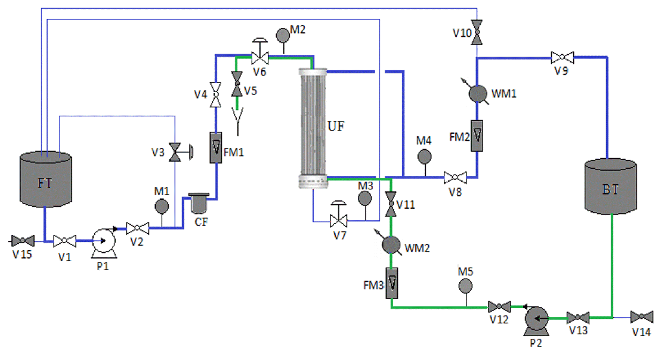
Schematic diagram of UF experimental set-up.
FT: Feed Tank. BT: Backwashing Tank. V1: Ball Valve. V3: Needle Valve. P1: Feed Pump.
P2: Backwash Pump. M1: Manometer. FM: Float Flow-Meter. CF: Cartridge Filter. WM1: Water Meter. UF: Ultrafiltration Membrane.

Membrane Specifications
During filtration, seawater is fed from the feed tank (FT) by a feed pump (P1). It passes a 50 μm cartridge filter (CF) and the flow-meter FM1. The feed, retentate and permeate pressures are measured respectively by the M2, M3, and M4 manometers. The retentate is recycled to the FT and the permeate volume is measured by the water meter WM1 then collected in the backwash tank BT.
During backwash steps, permeate is pumped from the backwash tank by P2 pump and enter the UF module in out/in configuration. The backwash flow and pressure are measured by the flow meter FM3 and the manometer M5, respectively. The water meter WM2 measures the volume of the consumed water during backwash. The water used for backwash is discharged.
The difference between the produced water (permeate) indicated by WM1 and consumed water (for the backwash) measured by WM2, is the Net Water Production (NWP).
The filtration experiments have been executed during 10 h at feed flow and pressure of 30 L.min−1 and 1.05 bar, respectively. These conditions have been chosen as they ensure a maximal conversion rate and minimal permeate turbidity (0.2 NTU) [29].
The flow circulation in the membrane fibers is laminar with Reynolds number of 410 and cross flow velocity of 0.5 m.s−1.
2.1. Fouling Mechanism Identification
The fouling mechanism during seawater ultrafiltration was first identified by modeling the flux decrease using the individual models of Hermia [5]. These models are chosen as they are simple and the required conditions of their use in cross flow filtration are available (cross flow filtration before steady state at laminar flow regime). Hermia [5] proposed four models describing fouling mechanisms responsible of flux decline under constant pressure filtration. The analytical expressions are recapitulated in Table 3. The four models are described in a unified equation as follow:
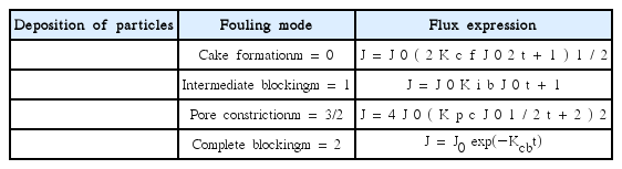
V : permeate volume (m3), t: filtration time (s).
K : Hermia model constant related to the nature of fouling (Ksb: standard clogging constant, Kcb: complete blocking constant, Kib: intermediate blocking constant, Kcf: cake formation constant).
m: characteristic value of each model: cake filtration m = 0, intermediate blocking m = 1, pore constriction (called also standard blocking) m = 3/2, and complete blocking m = 2.
Cake formation occurs when the pores of the membrane are smaller than the size of the particles present in the raw water. This deposit forms a porous layer generating additional resistance. Complete clogging assumes that each particle reaching the membrane blocks a pore. Intermediate clogging is based on the probability of open pores clogging or particles deposition on previously clogged pores. Standard blocking involves the adsorption of smaller particles onto the inner walls of the membrane pores by decreasing their volume and increasing the hydraulic resistance.
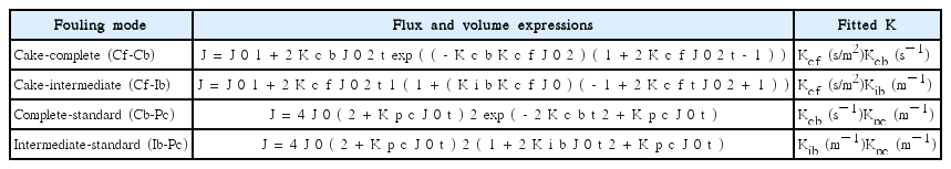
Moreover, the combined models of Bolton et al. [26] which join two different individual fouling mechanisms (pore blocking, pore constriction, caking) were also applied to consider the possibility of clogging mechanisms combinations during seawater UF. Initially these models were tested with biological fluids, and, they are extended to seawater in this work. Table 4 summarizes the flux expressions of the combined models which are derived from the volume expressions given in [26].
The fouling mechanisms responsible of flux decline were identified following the approach described in [30]. We considered the flux expressions relative to the individual and combined fouling mechanisms and the least square method to study the correlation between the experimental data and the theoretical models. As a result, optimized values of K with minimal value of least square are obtained for each model. An average error percentage was then calculated as:
Where Jexp and Jmodel are respectively the experimental and the predicted permeate flux.
The expression that best describes the experimental data suggests the most probable fouling mechanism responsible of the observed flux decline.
2.2. Experimental Design
An experimental screening study was done to establish the “weight” of the backwash parameters, to classify them and therefore to be able to choose -among them-those that are the most influential for a finer further optimization. The screened parameters were limited to the Backwash interval (BWI), the Backwash duration (BWD), the Backwash pulses (BWP), the Backwash Sodium hypochlorite injection (Inj), and the Backwash flow rate (BWF). The parameter levels are summarized in Table 5.

The Factors and Their Levels
The effects of these operating parameters were studied on three responses (Y1, Y2 and Y3):
Y1 is the irreversible fouling during the full operation time; it’s calculated as mentioned in ref. [31]:
J0 : Initial permeate flux of the filtration (L.h−1.m−2)
Ji(n+1) : Permeate flux at the beginning of the last filtration cycle (L.h−1.m−2)
Y2 is the reversible fouling during the full operation time; it’s calculated as mentioned in [31]:
Jf(n): Permeate flux at the end the penultimate cycle (L.h−1.m−2)
Y3 is the net water production (liter) expressed as the difference between the overall produced water and that used in backwashing phases.
The screening plan is generated using the Nemrodw® design software and consists of 25 experiments. The conditions and the results of those experiments are represented in Table 6. All experiments consist on a successive filtration-backwashing phases done during 600 min (10 successive hours) by applying backwashing at regular intervals of 30 or 60 min. Fig. 2 shows the evolution of the permeate flux for an experiment with 60 min filtration duration. Initially, the membrane is clean; the permeate flux is constant. During the filtration, it decreases and the backwash allows its restoration (because the fouling is not severe). After several filtration cycles, a simple backwash cannot restore the initial value of the permeate flux.

Uncoded Design Table for the Factors and Responses

The mathematical model used to study the relationship between responses and factors is a first order polynomial model:
where Y is the theoretical response, bi/j are the theoretical model coefficients corresponding to the relative influence of each variable on the response. i (1, 2, 3, 4 and 5) is the factor number and j (A, B, C and D) is the difference between a factor level and its last level (A is the difference between the first and the last level, B is the difference between the second and the last level, C is the difference between the third and the last level, D is the difference between the fourth and the last level). For example (b2/A: i = 2 = second factor BWD and j = A = difference between level 1 and the last level 4). X as mentioned in table 5 is the factor.
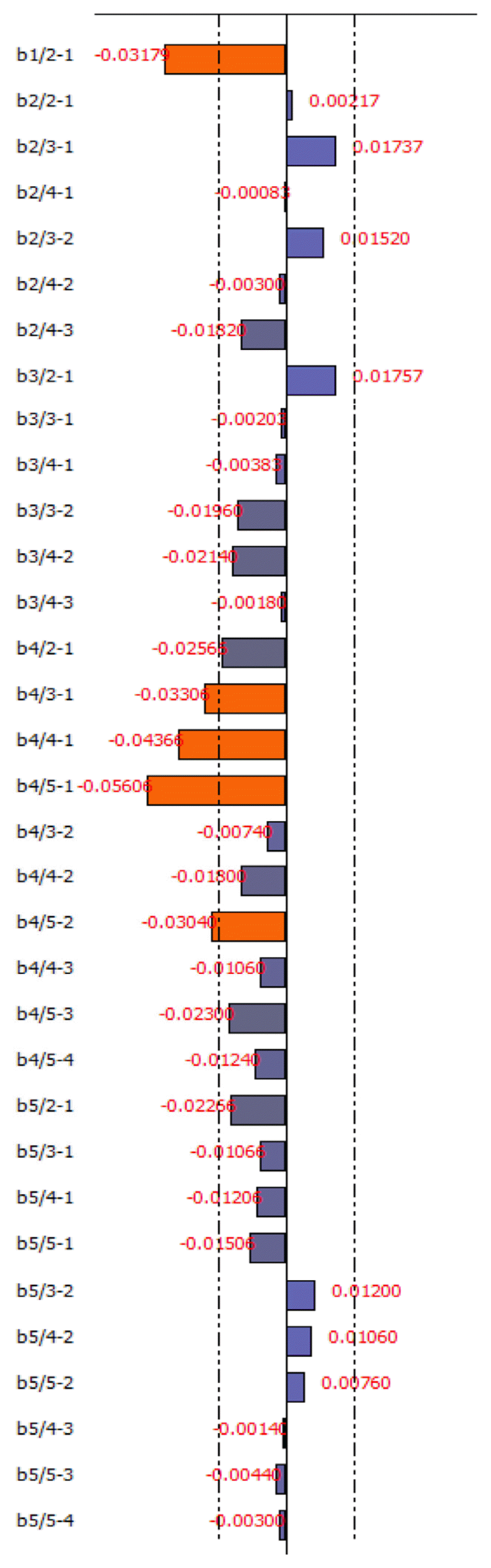
From the experimental data, the estimations of bi/j coefficients are calculated by the Nemrodw software. Each coefficient represents the effect of the corresponding factor (factor number i) when it varies from one level to another (represented by j). The choice of a factor as important or not depends on its effect on the response (statistically significant or insignificant). The significance of each coefficient is evaluated by student’s test (at 95% confidence level). The corresponding P-value must be less than 0.05 to ensure significance. The calculated effects can thus, be represented on bar chart (Fig. 5). We consider that if bi/j exceeds the significance level (represented by the dashed line in Fig. 5) the effect of this parameter is statistically significant.
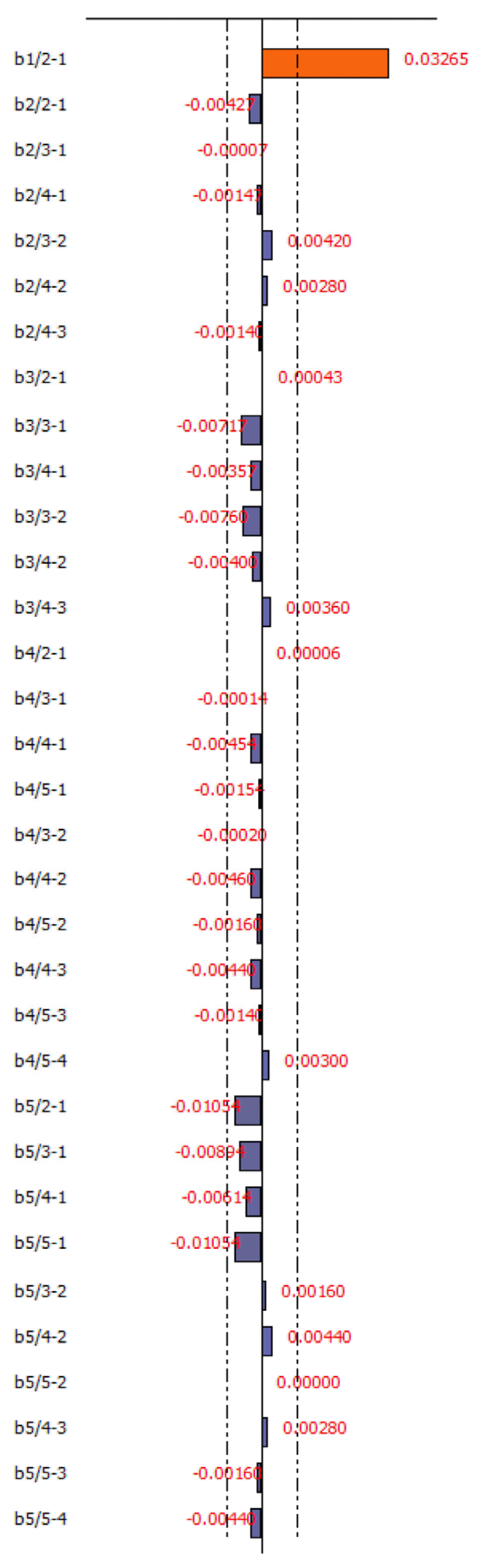
Bar chart of the factors: Effects on the reversible fouling response. (Nemrodw software)
3. Results and Discussion
3.1. Fouling Mechanisms Identification
The organic matter present in seawater can be particulate (colloids, particles, microorganisms, etc.) or dissolved (humic susbtances, low molecular weight neutrals, building blocks, low molecular weight acids and biopolymer) [1, 32]. Particulate matter is the main cause of UF membranes fouling; the 100 kDa membrane used in this work effectively retains suspended matter and reduces the turbidity of 4.4 in feed seawater at less than 0.21 in the permeate water and this, no matter what the operating conditions used during the backwash. Dissolved organic matter, in particular the biopolymer, even if it is poorly retained, can also contribute to the fouling of the 100 kDa membrane [32].
The identification of the fouling mechanism was performed for the experiments of 60 min backwash interval generated by the experimental design (Table 6). The classical models of Hermia and the combined models of Bolton were both used as previously described in the section “Fouling Mechanism identification”. The K and the % average error were estimated for each cycle of the 10 experiments (100 cycles were analyzed).
Considering that the results are similar for all experiences, only the results obtained for experiment 6 are presented in this section. Fig. 3 shows the fitting of Hermia models to experimental data for cycle 4 of experiment 6.
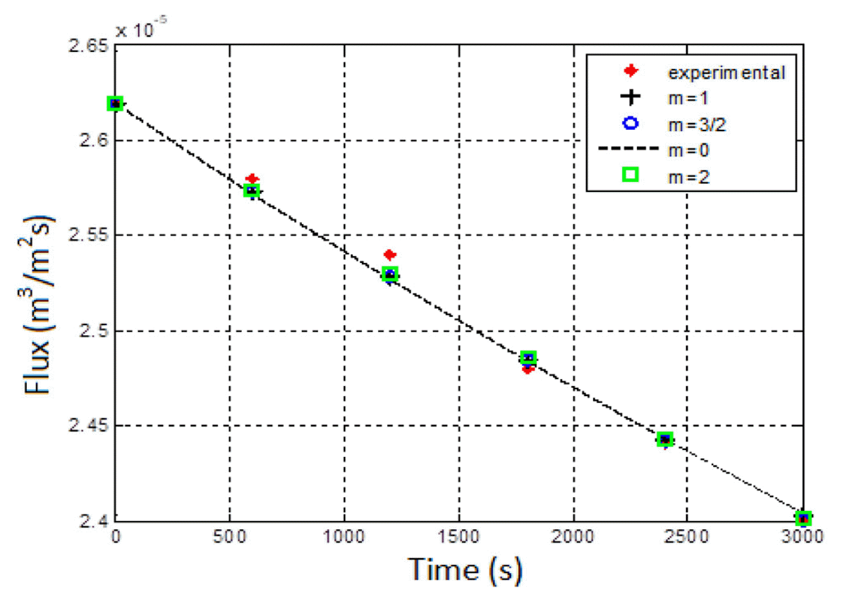
Variation of permeate flux versus time: Experimental data and Hermia models for experiment N°6 (cycle 4).
For a better analysis of the curves, the optimized values of K and the values of the average error of the flux prediction obtained after modeling are summarized in Table 7. Comparing Hermia and Bolton models, we have observed that the highest deviation between the experimental and predicted flux values is observed for the intermediate-standard (Ib-Pc) model with % average error ranging between 1.41% and 2.88%. The other combined models do not show better adjustments than Hermia models.

The Values of % Average Error and Estimated K for the Hermia and Bolton Models - Experiment 6 (BWI = 60 min. BWF = 22.5 L/min. BWD = 10 s. BWP = 2. Inj = 4.5 ppm)
Moreover, it can be seen that the error percentages are very close for the four Hermia mechanisms. It seems that no dominance of one mechanism over the other can be suggested in this case to describe the decrease in flux. Via et al. [21] and Torkamanzadeh et al. [15] also obtained very close or similar R2 values for the four Hermia models in the tangential ultrafiltration of polyethylene glycol and wastewater, respectively. In the case of a good fit (high R2), Torkamanzadeh et al. [15] concluded that the decrease in flow can be described by one of the four models because it seems that all the mechanisms coexist. In our case, this coexistence of mechanisms might be due to the feed complexity and the large distribution of the particles sizes (from 1 nm to 1 μm) as well as in the polymers (from 20 to 80 kDa) or in biologically active organisms. This can cause a synergistic fouling by internal clogging, pore blocking and cake formation [1, 33]. On the other hand, it may be assumed that cake formation might dominate for longer filtration cycles (more than 60 min) after pores have been blocked.
A simulation based on Hermia models was performed to predict the dynamic behavior of the permeate flux over an interval of 250 min for experiment 6, cycle 6 (Fig. 4). For 60 min filtration cycles, the Hermia models concordance is almost total; the gap widens for longer cycle durations.

Permeate flux evolution versus time for Hermia models (experiment 6. cycle 6).
Zone a: experimental data are in concordance with whatever Hermia’s model.
Zone b: higher than 60 min fouling can be described by a specific model of Hermia.
To go further in this approach, a Taylor approximation study was carried out to estimate the time interval in which the four models are superposed. The Taylor approximation would convert Hermia function to a series of polynomials representing the evolution of flux versus time. Table 8 represents the second degree Taylor polynomials of Hermia models in the case of experience 6, cycle 6. Eq. (6) allows us to estimate the time below where no difference between models is observed.

Taylor Approximation of Hermia Models
TD represents the Taylor development of Hermia model. i and j correspond to the designation of the Hermia model approximation and ɛ is the error.
For time less than 27 min, all the approximation equations (Table 8) are equal. However, the time is longer for the models: pore constriction and intermediate blocking. The difference between TDpc and TDib is observed after 45 min.
For 60 min filtration duration, the difference is still weak as the error is lower than 0.1% and doesn’t allow us to privilege one fouling mode rather than another.
3.2. Screening Study
The screening study is a strategy used to identify among a series of factors those which are the most influential on fouling and productivity. The design was established to screen 5 factors (the BWI, the BWD, the BWP, the Backwash Sodium hypochlorite injection (Inj), and the BWF) supposed to have an influence on the fouling of seawater UF. The effect of those parameters was studied on both reversible and irreversible fouling as well as on net water production.
3.2.1. The fouling
Fig. 5 and 6 show that the filtration duration is the main influential parameter on both reversible and irreversible fouling since the bars corresponding to its coefficients (b1/2-1) exceed the meaning limit (dashed line). However, it has significant opposite effects on the two responses. Its effect is positive on reversible fouling and negative on irreversible fouling. This means that as the filtration time increases from 30 to 60 min, reversible fouling becomes more important, as opposed to irreversible clogging. In other words, when the filtration time is longer (60 min), the irreversible fouling takes longer to settle. This assumes that external fouling mechanisms (complete blockage or cake formation) are the dominant mechanisms. The layers of particles formed on the surface of the membrane prevent severe internal clogging. For operation at 30 min, a more severe clogging seems to be more dominant because the cake layer does not have time to form (the cycle is short). Unfortunately, those hypotheses could not be confirmed in the fouling mechanism identification section. However, they are consistent with the work of Hwang et al. [3]. They believe that an extension of the filtration cycle length favors the formation of a layer of cake that would prevent internal blockage of the membrane pores. This cake layer, which is easily removed by backwashing, delays the appearance of irreversible clogging.
Bar chart of the factors: Effects on the irreversible fouling response. (Nemrodw software)
Moreover, the irreversible fouling is greatly affected by the hypochlorite concentration. A significant decrease in the irreversible fouling appears when the hypochlorite is injected at a concentration of 4.5 ppm (b4/3-1). The irreversible fouling continues to decrease when the hypochlorite concentration increases from 4.5 to 10 ppm (b4/4-1 and b4/5-1). This is expected because higher hypochlorite concentration can inhibit the growth of micro-organisms and oxidize more organic matter which reduces the irreversible fouling.
The backwash duration, backwash pulses and backwash flow rates don’t have significant effects on the fouling in the studied experimental domain.
3.2.2. The net water production
Fig. 7 shows that three factors (backwash interval (b1), backwash duration (b2) and backwash flow-rate (b5)) have significant effects on the response.

Bar chart of the factors: Effects on the net water production response. (Nemrodw software)
Backwash duration is the most influential factor on the response; there is a linear relationship between the increase in the backwash duration and the decrease in the net water production. Its increase from 10 to 20 (b2/2-1), 10 to 30 (b2/3-1) and 10 to 40 (b2/4-1) leads to a continued decrease in the net water production. This decrease in production is caused by a higher consumption of permeate during backwashing.
Filtration duration also has a significant effect on net water production with its coefficient b1/2-1 of a positive value of 86.8. This means that the longer the filtration time (30 to 60 min), the higher the net water production will be. Pervov et al. [34] and Xu et al. [35] agree that prolonged filtration duration up to a certain value would increase the net product water as the backwash is less frequent and the consumed permeate water is reduced. However, beyond this value, increasing the filtration duration leads to the contrary to reducing the NWP due to a more pronounced irreversible fouling. 60 min filtration duration which seems to be a good choice for seawater ultrafiltration as the irreversible fouling and the consumed permeate water were both minimized.
The results don’t show any significant effect on net water production when the backwash flow rate increases from 15 to 17.5 L.min−1 (b5/2-1). A significant decrease in net water production is observed when the backwash flow increases to 20 L.min−1 (b5/3-1) and reaches its highest value when BWF reaches 22.5 L.min−1 (b5/4-1) (Fig. 7). This is expected because bigger backwash flow consumes more permeate water without acting on reversible and irreversible fouling. No further decrease in the net water production is observed when the BWF increases from 22.5 to 25 L.min−1.
Backwash pulses and the hypochlorite concentration don’t have significant effects on the net water production in the studied experimental domain.
4. Conclusions
This work deals with the use of UF as seawater pretreatment prior to RO. With the aim of controlling and automatically regulating the clogging during seawater UF, it appeared necessary to identify the fouling mechanism and the influential parameters acting on it. This paper was conducted on two main axes. In the first one, we studied the fouling mechanism during UF using mathematical models describing clogging: Hermia models and Bolton combined models. The simulation shows that Bolton models combining two fouling mechanisms didn’t bring better results than the Hermia ones as the fitted curves are similar and the average error percentages are very close for all the models.
In the second part, the screening study was conducted to identify the most influential parameters on the fouling and the net water production. Five parameters were screened (the backwash interval, the backwash duration, the backwash flow-rate, the backwash pulsations, and the concentration of hypochlorite injected during backwashing). The results showed that both reversible and irreversible fouling were mainly affected by the filtration duration. Extending the filtration duration to 60 min led to a significant increase in the reversible fouling and significant decrease in the irreversible one because of a thicker cake layer formation which prevents severe internal fouling. The irreversible fouling is also significantly affected by the hypochlorite injection concentration; it decreases significantly and linearly with the hypochlorite concentration increase from 4.5 to 10 ppm. On another hand, the net water production is significantly influenced by the filtration duration, the backwash duration and the backwash flow rate. It increases when BWI increase from 30 to 60 min and linearly decreases when BWD increase from 10 to 40 s. The augmentation of the BWF from 15 to 20 L.min−1 or more also engenders a significant decrease in the net water volume.
It emerges from this study that the backwash interval, the backwash duration, the backwash flow, and the hypochlorite concentration are the most influents parameters that control the fouling and the productivity. As the influents factors have different effects on the responses, further work is needed to optimize the process and find compromise conditions to get large net water production for minimal fouling and cost consumption.
Acknowledgments
This work was made within a convention between the Tunisian Company of Electricity and Gas (STEG) and the LAMSIN. The authors would like to thank Mr. Mondher Haddaji, the plant operators and Mrs. Selima Allouche for their help, and the STEG as well as the LAMSIN for the financial support of the pilot construction.