Prediction of carbon dioxide emissions based on principal component analysis with regularized extreme learning machine: The case of China

Article information

Abstract

1. Introduction

After over 30 y of the economic reforms in China, there emerges a remarkable rise with average annual GDP growth rate at nearly 10% [1]. However, the burgeoning development of economy inevitably results in the large increase in energy consumption and hence CO₂ emissions. China overtook the United States as the world’s leading emitter of CO₂ in the year of 2006 [2]. To respond to the cause of serious global warming, China commits to continue taking effective measures for CO₂ emission control during the 13th Five-Year Plan, thus the carbon emission peaking can be reached by 2030. Accordingly, it’s of great significance to focus on CO₂ emissions prediction research, which provides a valuable reference for practical measures of CO₂ emission reduction.

A report published by the National Petroleum Council in the United States predicted a 50% – 60% growth in total global demand for energy by 2030 [3]. Energy consumption is the main source of CO₂ emissions [4], thus a lot of researchers have paid attention to this area. Say and Yucel [5] studied the relationship between total energy consumption and total CO₂ emissions through regression analysis, which displayed a strong relationship between these two factors. In [6], the energy consumptions were modeled using artificial neural network (ANN) based on economic and demographic variables. The results showed that the correlation coefficients between ANN predictions and actual energy consumptions were higher than 90%, which indicated a high reliability of ANN for forecasting future energy consumption. Azadeh and Tarverdian [7] presented an integrated algorithm based on genetic algorithm, computer simulation and design of experiments using stochastic procedures for monthly electrical energy consumption prediction. In [8], Utgikar and Scott explored the possible causes of inaccuracy in energy forecasting which could provide a better understanding of prediction process and design a strategy for reducing the errors in energy prediction. Aydin [9] utilized multiple linear regression analysis to study the relationship between CO₂ emissions and energy-related factors where correlation analysis were employed to determine the influential factors. In [10], an approach was proposed for coal-related CO₂ projections in future planning, wherein coal-related CO₂ emissions were modeled by trend analysis. Feng and Zhang [11] conducted a case study to predict the effects of different development alternatives on future energy consumption and carbon emission, namely under three scenarios: business-as usual, basic-policy and low-carbon. The results provided insights into the energy future and highlighted possible steps to develop a sustainable low-carbon city.

At this stage, researches on carbon emissions can be mainly divided into two parts: discussion on influential factors and study on prediction models. For the influential factors, existing studies related to this part include the methods such as index decomposition means [12–13] and input-output structural analysis [14–15]. Andres and Rustemoglu [16] introduced refined laspeyres index method into the research of relationships between CO₂ emissions and four identified factors in Brazil and Russia for the period 1992–2011 to explore the determinants of accelerating CO₂ emissions. Li et al. [17] applied logarithmic mean divisia index method (LMDI) to decompose the change in carbon emissions into some influencing factors caused by urbanization. The results revealed that energy intensity contributed largely to carbon emission reduction in Hubei Province. Li et al. [18] estimated the agricultural CO₂ emissions in China during the period of 1994 to 2011 and applied LMDI as the decomposition technique. The results illustrated that agricultural subsidy acts to reduce CO₂ emissions effectively and has increased in recent years. Wang et al. [19] proved that economic development, energy structure and low energy efficiency are three main driving factors of increasing CO₂ emissions in China based on a modified production-theoretical decomposition analysis approach. Ahmed [20] studied the relationship between CO₂ emissions, economic growth, urbanization and trade openness by two steps: (a) Autoregressive distributed lag bounds test was carried out to explore whether there existed co-integration between the variables. (b) The relationship between the factors was analyzed according to the long-run and short-run dynamics. Based on the last research, Ali et al. [21] added the factor of energy consumption to examine its dynamic impact on CO₂ emissions. Deng et al. [22] combined structural decomposition analysis and logarithmic mean divisia index method to study the drivers behind CO₂ emissions in Yunnan province. This technique could take both production and final demand into account in less-developed regions. Cointegration and Granger causality were adopted by Tang and Tan [23] to examine the relationship among CO₂ emissions, energy consumption, foreign direct investment and economic growth in Vietnam. They pointed out that there existed long-run equilibrium among these variables. Lin et al. [24] evaluated the relation between CO₂ emissions and industrial growth through an autoregressive distributed lag bounds testing and cointegration analysis. The results suggested that there was a reduction potential of CO₂ emissions in the Chinese manufacturing sector without intimidating industrial growth. Wang et al. [25] applied a two-level decomposition model based on Kaya identity to uncover the main influential factor for CO₂ emissions. The results indicated that energy intensity reduction was conducive to low-carbon economic development. Based on combining correlation analysis, gray correlation analysis and principal component regression analysis, Bian et al. [26] integrated data envelopment analysis with energy structure adjustment to measure CO₂ emission reduction in China. The findings showed that it was a practical way to decrease CO₂ emissions through the abatement of coal consumption and development of non-fossil energy.

For the forecasting techniques, CO₂ emissions are predicted mainly through the relationship models between carbon emission and its influencing factors based on different scenarios. Kang et al. [27] employed STIPRAT model to examine the impact of energy-related factors on CO₂ emissions and tested the spillover effects of per capita CO₂ emissions through a spatial panel data technique. This study provided some policy advice on reduction of China’s CO₂ emissions. Based on STIPRAT model, Sheng and Guo [28] extended this basic method to be a panel error-correction one which can dynamically take the influence of urbanization changes on total CO₂ emissions into consideration. Their findings indicated that the rapid urbanization augmented CO₂ emissions both in the short-run and long-run. Wu et al. [29] utilized a multi-variable grey model to forecast CO₂ emissions on the basis of energy consumption, urban population and economic growth. Pérez-Suárez et al. [30] compared environmental kuznets curve with logistic growth model in CO₂ emission prediction considering a sample of 175 countries. The results showed that extended environmental kuznets curve tended to outperform the forecasting accuracy of the latter one. Vector autoregressive model was adopted by Xu and Lin [31] to identify the drivers of CO₂ emissions in China’s iron and steel industry. The findings revealed that energy efficiency played a significant part in CO₂ emission reduction. Baareh [32] introduced four input data including oil, natural gas, coal and primary energy consumption to build ANN for CO₂ emission prediction. The results proved ANN was a powerful and efficient tool in forecasting CO₂ emissions. A hybrid model that combined ANN with bees algorithm for analyzing CO₂ emissions in the world was presented by Behrang et al. [33]. Two steps were carried out: (a) The bees algorithm was applied to determine the indicators. (b) World CO₂ emissions were forecasted up to the year of 2040 based on ANN.

With the propositions and prosperities of artificial intelligent algorithms, traditional neural networks offer a new way of CO₂ emission prediction. Despite their strong nonlinear mapping ability and parallel processing capability, the drawbacks of these methods are the slow learning speed, complex training parameters and easily tapping into the local minimum. Huang et al. [34] introduced extreme learning machine (ELM) to solve the stated issue of conventional training methods. With the advantages such as fast convergence speed, high training accuracy and no manual tuning, the ELM model has been successfully applied to forecasting problems in many fields, such as wind speed [35], electricity load [36], oil price [37] and so on. However, ELM is based on empirical risk minimization principle which easily causes over-fitting phenomenon. Therefore, in order to guarantee the global optimization and generalization ability, regularized extreme learning machine (RELM) model, in which the calculation process of Moore-Penrose generalized inverse and the introduction of the regularization factor are added to ELM, is used for CO₂ emission prediction in this paper.

In general, based on the aforementioned studies, it can be found that the appropriate selection of influential factors has momentous influence on the prediction results of CO₂ emissions. However, most studies only put emphasis on the impact of these factors on the total CO₂ emissions and ignore the correlation to each other. In reality, there exist overlaps of information contained in the data, thus, the computational efficiency is greatly depressed due to the complex network. Therefore, principal component analysis (PCA) is employed in this paper to reduce the dimension of pre-select influential factors with retention of information to the utmost so that the network structure can be simplified and operation efficiency and prediction accuracy can be significantly improved.

Therefore, compared with past works, there exist two main differences: (i) RELM, a new kind of neural networks, is firstly introduced into CO₂ emission prediction, which overcomes the disadvantages of slow learning speed, the need of numerous training samples, over-fitting and so on in the previous researches. (ii) The correlations among influential factors are paid close attention in this paper, thus PCA is utilized to manipulate them for dimension reduction to improve the computational efficiency and forecasting precision. The rest of this paper is organized as follows: Section 2 presents a brief description of PCA, ELM and RELM; Section 3 displays the framework of the proposed novel approach in this study; Section 4 elaborates the selection of input; Section 5 validates the established model through a case study; Finally, the paper is concluded and several concrete mitigation measures have been further put forward in Section 6.

2. Methodology

2.2. Extreme Learning Machine

The ELM is a novel machine learning algorithm for single layer feed-forward neural networks. The main nature of ELM is the random initialization of the input weights and hidden biases without iterative adjustments during the learning process, thus the optimal output weights can be quickly obtained based on the predefined network structure [40]. Besides its fast learning speed, ELM also avoids numerous problems such as local minima and learning rate faced by other ANNs [41]. The topological structure of ELM network is illustrated in Fig. 1. The specific procedures of ELM are described as follows:

Fig. 1

The ELM network.

Given a training data set with N samples {(x_i, y_i )}_i=1^N, the ELM model with L hidden nodes are expressed as

(1) ∑i=1Lβig(wi·xj+bi)=yj,         j=1,2…,N

where x_j is the input pattern, y_j is the desired output, w_i∈R is the randomly assigned input weight vector between the ith hidden node and input nodes. b_i is the randomly selected bias of the ith hidden node. g(·) is an activation function. β_i represents the weight connecting the ith hidden node and output nodes.

The Eq. (1) can be simply written as:

(2) H β=y

where

(3) H(w1,…,wL,x1,…,xN,b1,…,bL)=[g(w1·x1+b1)…g(wL·x1+bL)   ………   g(w1·xN+b1)…g(wL·xN+bL)]N×L

(4) {β=[β1T,…,βLT]y=[y1T,…,yNT]

The output weights can be derived by finding the least square solutions to the linear Eq. (5):

(5) ‖H β-y‖=‖HH+y-y‖=minβ‖H β-y‖

Here the least square solutions are obtained as follows:

(6) β=H+y

where H⁺ represents the Moore-Penrose generalized inverse matrix of hidden layer output matrix H.

3. Approaches of PC-RELM Model

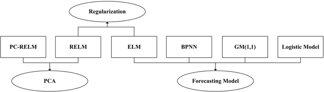
The framework of the proposed model for carbon dioxide emission prediction is displayed in Fig. 2. This novel approach can be explained in detail as follows:

Fig. 2

Framework for carbon dioxide emission prediction based on PC-RELM.

In part I, the Pearson coefficient analysis and bilateral significance test are carried out to study the relationships between the impact factors and carbon dioxide emissions. The partial autocorrelation analysis is adopted to select historical carbon dioxide emissions with highest correlation on the target emission. This section contributes to the pre-selection of input for research. In part II, PCA is employed for feature extraction and dimension reduction of the pre-selected data, which can improve the computational efficiency. Part III aims at realizing carbon dioxide emission prediction through RELM model.

4. Input Selection

4.1. Data Source and Conversion

The research is made based on energy consumption as well as other related data in China from the year of 1978 to 2014. The consumption of total energy and percentage composition of four kinds of energies that contain raw coal, crude oil, natural gas and primary electricity are recorded in China Statistical Yearbook on the basis of standard coal. Considering there is no direct promulgation of CO₂ emissions, conversion coefficients listed in Table 1 are employed to convert the standard coal data to corresponding values of CO₂ emissions, according to the comprehensive report of “China sustainable development of energy and carbon emission scenarios analysis” [44]. The yearly CO₂ emissions in China during the period 1978–2014 are shown in Table 2.

Table 1

CO₂ Emission Conversion Coefficients for Different Energy Species

Table 2

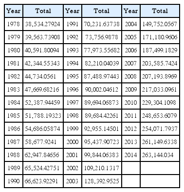
CO₂ Emissions over the Period of 1978–2014 in China (10,000 tons)

In Fig. 3, it can be clearly found out that there exists a continuous rise in CO₂ emissions of the total one, which displays the same trend with raw coal. This is due to the fact that coal is the main fuel in China which accounts for nearly 65% in primary energy consumption structure. However, crude oil and natural gas contribute a relatively small proportion of CO₂ emissions. Fig. 4 displays the growth multiple of CO₂ emissions of different energies from 1979 to 2014 with the data in 1978 as the base. The trend can be divided into two stages: there was a gentle rise with slow growth rate before the year of 2002. After this turning point, the growth rate increased rapidly and the growth multiple reached about 6.8 in 2014. Moreover, in response to the national call for energy conservation and emission reduction nowadays, the utilization of natural gas is vigorously promoted. This is the main reason why natural gas presents a significant increase in CO₂ emissions in recent years.

Fig. 3

CO₂ emissions of total energies and main sources during 1978–2014 in China.

Fig. 4

CO₂ emission growth multiple of of total energies and main sources.

4.2. SPSS Analysis

In the previous studies on carbon dioxide emission forecasting, influential factors mainly contain energy consumption, GDP, population, urbanization rate, service industry and so on [45–48]. In this paper, eleven variables are pre-selected from China Statistical Yearbook for CO₂ emissions prediction including coal consumption, GDP of primary industry, GDP of secondary industry, GDP of tertiary industry, population, urbanization level, transportation possession quantity, power generation, steel production, total investment in fixed assets of the whole society and area final consumption.

Mining the relationships between CO₂ emissions and the eleven pre-selected variables are essential for the establishment of a good prediction model. Pearson coefficient and bilateral significance test are selected for correlation analysis in this paper. Table 3 presents the values of correlation coefficients. It can be found that all the correlation coefficients are more than 0.8 and the concomitant probability value of bilateral significance test is 0.000 less than 0.05, which reveals that there exists positive and significant correlation between CO₂ emissions and the eleven above-mentioned indicators. Thus, the eleven pre-selected variables all should be taken into account in the CO₂ emission prediction.

Table 3

Correlation Analysis at the Bilateral Significance Level of 0.01

4.3. PACF Analysis

The influence of historical CO₂ emissions on the target one is taken into consideration in this part. PACF is employed to find out the inherent relationship of the dataset. The partial autocorrelograms is illustrated in Fig. 5, where the confidence level is 90%. The results indicated that carbon emssion data in lag 1 and lag 2 showed a strong correlation, thus these two variables are also selected as influential factors.

Fig. 5

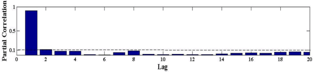
PACF of total CO₂ emissions dataset.

4.4. PCA Process

Based on the pre-selected thirteen variables in the section of 4.1 and 4.2, PCA is utilized to remove the multicollinearity presented in the predictors. We mine the major information containing in the data through this method. The PCA process result is shown in Table 4 and Fig. 6. It can be seen that the first principal component explain more than 95% of the factors, so this principal component is utilized to replace the predictors as the input.

Table 4

Component Matrix

Fig. 6

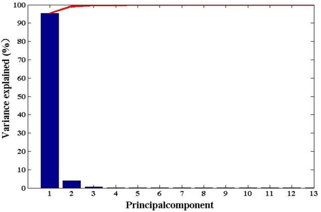
Scree plot in PCA analysis.

5. Experiment of CO2 Emission Prediction in China Based on RELM Model

5.1. Comparative Framework

The experiment of CO₂ emission prediction in China is carried out based on the aforementioned related data from 1978 to 2014, totally 37 data points. Wherein, the data from 1980 to 2009 are selected as training set and the remaining 5 data are utilized as test set.

As shown in Fig. 7, three comparative parts are contained in the framework. In part I, four basic models including ELM, BPNN, GM(1,1) and Logistic model are introduced to forecast CO₂ emissions. Part II utilizes RELM to test whether the regularization parameter donates to the prediction accuracy and the effectiveness of PCA is explored in Part III.

Fig. 7

Comparison framework for CO₂ emission forecasting.

5.3. Parameter Setting

As above mentioned, only two parameters need to be pre-set in RELM model. The regularization parameter C and the number of node in hidden layer are set as 2¹⁰ and 100, respectively. As compared models, the selection of parameters in ELM and BPNN is listed in Table 5.

Table 5

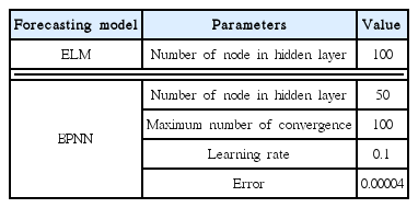
Parameters for ELM and BPNN Model

5.4. Results and Discussion

In Fig. 8, CO₂ emission prediction curves from 2010 to 2014 are obtained by six different models. It can be obviously found out that: (a) in contrast with other five models, the goodness of fit between the forecasted value by PC-RELM and actual value reaches the highest degree; (b) the fitting condition of ELM-based models is generally better than other techniques mainly due to the strong generalization ability; (c) the hybrid model PC-RELM presents higher predicted precision than RELM which indicates that the PCA part can effectively improve the prediction performance of the single RELM.

Fig. 8

CO₂ emission forecasting results from 2010 to 2014.

Fig. 9 displays the relative errors achieved by the six prediction models. The relative errors obtained by PC-RELM are all under 0.5% which outperforms other methods except in the year of 2011. The single RELM model exhibits a slightly lower error in the second point than PCA-RELM. In addition, there emerges large deviation between the actual values and predicted ones in BPNN and GM(1,1) model where the maximum relative errors are both over 9%.

Fig. 9

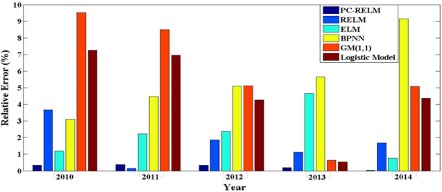
Comparison of relative errors for different forecasting models.

The statistical errors of the six forecasting techniques are clearly shown in Table 6. The analysis manifests that: (a) PC-RELM model provides the best prediction results in terms of MAPE, MaxAPE, MdAPE and RMSE. (b) Compared with RELM model, the PCA part in PC-RELM removes the multicollinearity in pre-selected influential factors and simplifies the network structure which contributes to the operation efficiency and the improvement of forecasting performance. (c) The errors of RELM is lower than ELM mainly due to the fact that the introduction of the regularization parameter in RELM enhances the global optimization and generalization ability of ELM model in CO₂ emission prediction. (d) Considering the significant influence of representative samples on BPNN, the MAPE, MaxAPE, MdAPE and RMSE values are higher than ELM-based algorithms. (e) The errors obtained by GM(1,1) are largest among the six models mainly because the smoothness degree of the original data has an impact on the prediction accuracy. (f) The prediction precision of Logistic model is higher than BPNN and GM(1,1) while it is remarkably lower than ELM-based models. The MAPE value of Logistic model is 18.5 times larger than PC-RELM.

Table 6

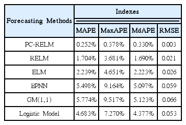
Statistical Error Measures of Prediction Methods

The computing time of PC-RELM, RELM, ELM and BPNN for continuously running for 100 times in MATLAB 2014a on a Windows 7 system is shown in Table 7. It can be clearly seen that ELM-based models save more computing time than BPNN model mainly because there is no need to update the randomly selected parameters in the learning process. In contrast with ELM, RELM takes 2.44 s for computing, which is slightly longer than ELM. Therefore, the regularization part has little impact on the running speed of ELM while improving the forecasting accuracy. Notably, PC-RELM is 0.3 s shorter than RELM, thus the PCA part can upgrade the running speed to some degree with the improvement of prediction precision.

Table 7

Computing Time of PC-RELM, RELM, ELM and BPNN Models

6. Conclusions

This paper chooses eleven influential factors including the lag phases of historical CO₂ emissions. After reducing the dimensionality of the influential factors through PCA process, RELM is introduced to forecast the CO₂ emissions. Several conclusions can be obtained as follows: (a) the PCA process is conducive to improving the operation speed and forecasting accuracy; (b) the high prediction precision of RELM model is attributed to the introduction of regularization part which enhances the global optimization and generalization ability with little time cost. (c) RELM combined with PCA outperforms other models with the lowest MAPE, MaxAPE, MdAPE and RMSE, indicating that PC-RELM model is a promising technique for CO₂ emission prediction.

Based on the findings in this paper, some suggestions for CO₂ emission reduction have been proposed with the consideration of selected influential factors: (a) According to the correlation analysis, coal consumption is completely correlated with CO₂ emission, thus it’s necessary to substitute fossil energy with renewable and clean energy so as to achieve the diversification of energy consumption. (b) The economic growth should rely on innovative talents and technological advancements to improve resource allocation efficiency. The proportion of primary, secondary and tertiary industry ought to be reasonably adjusted thereby reducing energy consumption of GDP per capita. (c) People should enhance their low carbon awareness and cut down energy consumption during their life and labor. (d) To control vehicle exhaust emissions, traffic restrictions based on even-numbered and odd-numbered license plates can be implemented to reduce pollutant emissions and traffic pressure.

Article information Continued