Carbon dioxide emissions, GDP per capita, industrialization and population: An evidence from Rwanda

Article information

Environmental Engineering Research. 2017;22(1):116-124

Publication date (electronic) : 2016 November 7

doi : https://doi.org/10.4491/eer.2016.097

Samuel Asumadu-Sarkodie, Phebe Asantewaa Owusu

Sustainable Environment and Energy Systems, Middle East Technical University, Northern Cyprus Campus, 99738 Kalkanlı, Güzelyurt, Mersin 10, Turkey

^†Corresponding author, Email: samuelsarkodie@yahoo.com, Tel: +90-5338213422

Received 2016 August 4; Accepted 2016 November 3.

Abstract

The study makes an attempt to investigate the causal nexus between carbon dioxide emissions, GDP per capita, industrialization and population with an evidence from Rwanda by employing a time series data spanning from 1965 to 2011 using the autoregressive distributed lag model. Evidence from the study shows that carbon dioxide emissions, GDP per capita, industrialization and population are co-integrated and have a long-run equilibrium relationship. Evidence from the Granger-causality shows a unidirectional causality running from industrialization to GDP per capita, population to carbon dioxide emissions, population to GDP per capita and population to industrialization. Evidence from the long-run elasticities has policy implications for Rwanda; a 1% increase in GDP per capita will decrease carbon dioxide emissions by 1.45%, while a 1% increase in industrialization will increase carbon dioxide emissions by 1.64% in the long-run. Increasing economic growth in Rwanda will therefore reduce environmental pollution in the long-run which appears to support the validity of the environmental Kuznets curve hypothesis. However, industrialization leads to more emissions of carbon dioxide, which reduces environment, health and air quality. It is noteworthy that the Rwandan Government promotes sustainable industrialization, which improves the use of clean and environmentally sound raw materials, industrial process and technologies.

Keywords: ARDL bounds test; Carbon dioxide emissions; Econometrics multivariate co-integration; Rwanda

1. Introduction

Climate change has become a global problem which has attracted attention from researchers and policy makers within the last decades [1]. This global phenomenon has been associated with the increasing demand of energy [2], the overdependence on fossil fuels [3], increasing population and poor agricultural practices [4]. “There has been a global rise of carbon dioxide emissions within the past 36 y (1979–2014) from 1.4 parts per million per year in earlier 1995 to 2.0 parts per million per year afterwards” [5]. As a result, there has been an immense contribution towards mitigating climate change and its impact, through the emergence of the Sustainable Development Goal (SDG-13) [1]. As outlined in the SDG-13, a global contribution towards climate change mitigation requires an incorporation of climate change measures into existing national policies, strategies and planning [6–8]. Climate change measures require a scientific and innovative research that provides evidence of the causal effect of environmental pollution and information for environmental policy makers, donor agencies and investors [9]. The emergence of modern econometric techniques has played an important role in providing a scientific proof of the causal effect of environmental pollution in different countries and continents. However, literature is limited in the case of Rwanda therefore, the study makes an attempt the empirically examine the causal nexus between carbon dioxide emissions, GDP per capita, industrialization and population.

The remainder of the study consists of literature review in section 2, methodology in section 3, results and discussion in section 4, while the conclusion and policy recommendation is in section 5.

2. Literature Review

A lot of studies have examined the causal effect of carbon dioxide emissions in different scope of studies. Majority of the existing literature can be categorized into three; the first category of research, Al-Mulali et al [10], Apergis and Ozturk [11], Balaguer and Cantavella [12], Bilgili et al [13], Hamit-Haggar [14], Kang et al [15], Lise and Van Montfort [16], Osabuohien et al [17], Saidi and Hammami [18], Seker et al [19], Shahbaz et al. [20], Shahbaz et al [21], Tutulmaz [22] examines the causal effect of environmental pollution, energy consumption and macroeconomic variables by testing the validity of the environmental Kuznets curve hypothesis. Al-MulaliSolarin and Ozturk [10] examined the relationship between carbon dioxide emissions, fossil-fuel energy consumption, GDP, urbanization and trade openness with a data spanning from 1980–2012. Their study found evidence of long-run and short-run causal relationship while supporting the validity of the environmental Kuznets curve hypothesis. Apergis and Ozturk [11] examined the validity of the environmental Kuznets curve hypothesis by employing a data spanning from 1990–2011 by using the generalized method of moments in Asia. Evidence from the study supported the validity of the environmental Kuznets curve hypothesis. AhmedShahbaz and Kyophilavong [23] examined the causal effect between carbon dioxide emissions, GDP and energy consumption in Brazil, South Africa, China and India using a panel data spanning from 1970–2013 using the fully modified least squares method. Their study confirmed the validity of the environmental Kuznets curve hypothesis and found evidence of bidirectional causality between carbon dioxide emissions and energy consumption.

The second category of research, Ahmed et al [23], Asumadu-Sarkodie and Owusu [24], Asumadu-Sarkodie and Owusu [25], Azhar Khan et al. [26], Chang [27], Fei et al. [28], Gul et al. [29], Saidi and Mbarek [30], Soytas and Sari [31], Cerdeira Bento and Moutinho [32], Menyah and Wolde-Rufael [33], Mohiuddin et al [34], Asumadu-Sarkodie and Owusu [35–42] examine the causal-effect of environmental pollution, energy consumption and macroeconomic variables without testing the validity of the environmental Kuznets curve hypothesis. Asumadu-Sarkodie and Owusu [37] examined the relationship between carbon dioxide emissions, GDP, energy use, financial development and population in the Sri Lanka by employing a data spanning from 1971–2012 using the ARDL approach and the neural network. There was evidence of a bidirectional causality between energy use and industrialization while there was a unidirectional causality running from carbon dioxide emissions to energy use. Asumadu-Sarkodie and Owusu [25] examined the causal nexus between carbon dioxide emissions, energy consumption, population and GDP in Ghana by employing a data spanning from 1980–2012 using VECM technique. Their study found evidence of a long-run equilibrium relationship between carbon dioxide emissions, energy consumption, population and GDP and a bidirectional causality between carbon dioxide emissions and energy consumption. Azhar Khan et al. [26] examined the long-run equilibrium relationship between energy consumption and greenhouse gas emissions by employing a panel data spanning from 1975–2011 in Sub-Saharan Africa, East Asia and Pacific, East Europe and Central Asia, South Asia, Middle East and North Africa, Latin America and Caribbean and the total world data. There was evidence of a long-run equilibrium relationship between greenhouse gas emissions and energy use. In addition, their study found an evidence of Granger-causality running from energy consumption to greenhouse gas emissions.

The third category of research, Asumadu-Sarkodie and Owusu [43], Dodder et al. [44], Li et al [45], Zou et al. [46] examine the causal-effect of environmental pollution and agricultural variables. Asumadu-Sarkodie and Owusu [43] investigated the relationship between carbon dioxide emissions and agriculture in Ghana by employing a data spanning from 1961–2012 using the VECM and the ARDL model. Their study found evidence of a long-run causal relationship between carbon dioxide emissions and agriculture in Ghana.

Evidence from the existing literature is inconsistent with each other and suggests that the outcome of the causal-effect of environmental pollution and macroeconomic variables vary from country-to-country and vary from one econometric technique to the other. The majority of the studies employ a panel data technique over time series data. In addition, there was difficulty in identifying a literature that has employed a time series data based on econometric techniques to examine the causal effect of environmental pollution and macroeconomic variables in Rwanda.

Rwanda, the “country of a thousand hills” is one of the smallest countries in east Africa [47]. UNDP [48] human development indicator ranks Rwanda in a low human development category with a human development index of 0.483, US$ 1,426 GDP per capita, 70.8% of the population in multidimensional poverty, 12.1 million populations and 0.1 tonnes of carbon dioxide emissions per capita. Nevertheless, the scientific evidence of the causal effect of carbon dioxide emissions, GDP per capita, industrialization and population have not been extensively investigated in Rwanda.

The study is in line with the work of Asumadu-Sarkodie and Owusu [24] who examined the causal nexus between carbon dioxide emissions, energy use, population growth and GDP in Ghana by employing a data spanning from 1971–2013 by comparing VECM and ARDL model. Their study found evidence of a bidirectional causality running from energy use to GDP and a unidirectional causality running from carbon dioxide emissions to GDP, population and energy use. In addition, evidence from their study shows that a 1% increase in population will increase carbon dioxide emissions by 1.72%. In contrast to their study, the present study makes an attempt to examine the causal nexus between carbon dioxide emissions, GDP per capita, industrialization and population in Rwanda with a data spanning from 1965–2011 by employing the autoregressive distributed lag approach. To meet the aim of the study, we examine the descriptive statistical analysis, unit root test, ARDL bounds test, ARDL regression, Granger-causality, impulse-response test, diagnostics and stability tests. As a contribution to literature, the study improves existing literature with the Rwanda case and further increases the global debate on climate change mitigation and its impacts from the Rwanda perspective. In addition, the policy recommendations emanating from the study will provide information on climate change policies, strategies and sustainable development planning in Rwanda.

3. Methodology

3.1. Data

The study attempts to examine the causal nexus between carbon dioxide emissions, GDP per capita, industrialization and population: An evidence from Rwanda by employing a time series data spanning from 1965 to 2011 using the Autoregressive Distributed Lag (ARDL) Model. Four study variables were employed from the World Bank [49] which include; CO₂ - Carbon dioxide emissions (kt), GDPPC-GDP per capita (current LCU), IND-Industry, value added (current LCU) and POP-population. It is noteworthy that industry value added is used as a proxy for industrialization since industry value added represents the contribution of public/private industries to the overall GDP [37].

3.2. Descriptive Analysis

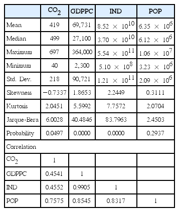
Table 1 presents the descriptive statistical analysis of the study variables. Evidence from Table 1 shows that CO₂ exhibits a long-left-tail (negative skewness) while GDPPC, IND and POP exhibit a positive skewness. Moreover, as CO₂ and POP exhibit platykurtic distribution, GDPPC and IND exhibit leptokurtic distribution. Evidence from the Jarque-Bera test statistic in Table 1 shows that except POP, CO₂, GDPPC and IND are not normally distributed at 5% significance level. In order to have a stable variance prior to the econometric analysis, the study corrects the variables by applying a logarithmic transformation. In order to prevent the problem of multicollinearity between the variables, the study examines the correlation between variables. Evidence from Table 1 shows that the strength of association is less than 0.900, meaning that no issue of multicollinearity exists between the variables. Fig. 1 shows the trend of the variables which increase periodically.

Table 1

Descriptive Statistical Analysis

Fig. 1

Trend of variables.

3.3. Model Estimation

The causal nexus between carbon dioxide emissions, GDP per capita, industrialization and population can be represented by a linear function expressed as:

(1) LCO2t=f(LGDPPCt, LINDt, LPOPt)

The empirical specification for the model is expressed as:

(2) LCO2t=β0+β1LGDPPCt+β2LINDt+β3LPOPt+ɛt

Where LCO₂_t is the logarithmic transformations of carbon dioxide emissions while LGDPP C_t, LIND_t and LPOP_t are the logarithmic transformationst of GDP per capita, industrialization and population in year t, ɛ_t is the error term and β₀, β₁, β₂ and β₃ are the elasticities to be estimated.

Following the work of Asumadu-Sarkodie and Owusu [24], Asumadu-Sarkodie and Owusu [43], the study employs the ARDL approach since is unbiased and has superiority over other econometric variables in small sample size. According to Pesaran and Shin [50], the ARDL model can be estimated with time series in a cointegration at either I(0) or I(1). The ARDL cointegration regression form for the study is expressed as:

(3) ΔLCO2t=α0+δ1LCO2t-1+δ2LGDPPCt-1+δ3LINDt-1+δ4LPOPt-1+∑i=1pβ1ΔLCO2t-i+∑i=0pβ2ΔLGDPPCt-i+∑i=0pβ3ΔLINDt-i+∑i=0pβ4ΔLPOPt-i+ɛt

Where α represents the intercept, p represents the lag order, ɛ_t represents the error term and Δ represents the first difference operator. The long-run equilibrium relationship between the series is examined using the F-tests based on the null hypothesis of no cointegration between LCO₂, LGDPPC, LIND and LPOP [H₀ : δ₁ = δ₂ = δ₃ = δ₄ = 0], against the alternative hypothesis of cointegration between LCO₂, LGDPPC, LIND and LPOP [H₁ : δ₁ ≠δ₂ ≠δ₃ ≠δ₄ ≠0].

The main purpose of using the ARDL model is to describe the factors (predictors) that can be changed to reduce carbon dioxide emission impacts in Rwanda while identifying the key predictors that influence each predictor [51].

4. Results and Discussion

4.1. Unit Root

As a pre-requirement, the study estimates the unit root test using Phillip-Perron’s (PP) and Kwiatkowski-Phillips-Schmidt-Shin (KPSS) test statistic based on the null hypothesis of a unit root and stationarity, respectively. The unit root tests (PP and KPSS) are used to test for the stationarity of the time series data in order to prevent spurious regression [52]. Evidence from Level in Table 2 shows that the null hypothesis of a unit root cannot be rejected in the PP test while the null hypothesis of stationarity is rejected at 5% significance level. Nevertheless, the evidence from First difference in Table 2 shows that the null hypothesis of a unit root is rejected in the PP test while the null hypothesis of stationarity cannot be rejected at 5% significance level, meaning that, the series are integrated at I(1).

Table 2

Unit Root Test

4.2. ARDL Regression Analysis

Once the pre-condition has been met, the study estimates the ARDL bounds test in order to examine the cointegration among the series. Cointegration is mostly used to examine the long-run equilibrium relationship among different variables. Using Akaike information criterion to select the optimal model for the bounds testing, Table 3 presents the results of the ARDL bounds test. Evidence from Table 3 shows that the F-statistics [8.49] is above the upper bound [3.77, 4.35, 4.89 and 5.61] at 10%, 5%, 2.5% and 1% significance level which shows a rejection of the null hypothesis of no cointegration between LCO₂, LGDPPC, LIND and LPOP.

Table 3

ARDL Bounds Test

Since the variables are co-integrated, the next step is to estimate the ARDL regression. Table 4 presents the ARDL regression. Evidence from Table 4 shows that the speed of adjustment (ADJ) [CO₂ L1. = -0.72] is negative and significant at 5% significance level, meaning that there is a long-run equilibrium relationship between variables running from LGDPPC, LIND and LPOP to LCO₂. Table 4 further shows evidence of the short-run equilibrium relationship between variables. The study applies the linear restriction test in order to estimate the joint effect of the individual outcomes at their various lags. Evidence from the joint estimate shows that there is a short-run equilibrium relationship between variables running from LIND to LCO₂ and LPOP to LCO₂. In addition, the study estimates the long-run elasticities which has policy implications. Evidence from Table 4 shows that a 1% increase in LGDPPC will decrease (inelastic) LCO₂ by 1.45%, while a 1% increase in LIND will increase (elastic) LCO₂ by 1.64% in the long-run.

Table 4

ARDL Regression

4.3. Granger-causality Test

Due to the inability of ARDL regression to estimate the direction of causality, the study employs the Granger-causality based of VECM to estimate the direction of causality among variables. Evidence from Table 5 shows that the null hypothesis that LIND does not Granger-cause LGDPPC, LPOP does not Granger-cause LCO₂, LPOP does not Granger-cause LGDPPC, LPOP does not Granger-cause LIND is rejected at 5% significance level. Meaning that, there is evidence of a unidirectional causality running from LIND → LGDPPC, LPOP → LCO₂, LPOP → GDPPC and LPOP → LIND.

Table 5

Granger-causality

4.4. Impulse-response Analysis

The Granger-causality is limited to testing the direction of causality among series but fails to examine how the variables respond to random innovations in other series. The study employs the impulse response analysis which prevents the orthogonal problems associated with out of sample Granger-causality tests. Evidence from Fig. 2 shows that the response of LCO₂ to LPOP, LGDPPC to LPOP and LIND to LPOP are insignificant within the 10-period horizon. In contrast, the response of LCO₂ to LGDPPC and LIND is significant and gradually increases with a constant trend within the 10-period horizon. Hence, contrary to the evidence of the Granger-causality, the evidence from the impulse-response shows that GDP per capita and industrialization affects carbon dioxide emissions in a 10-period horizon in Rwanda.

Fig. 2

Impulse response of variables to each other.

Moreover, the response of LGDPPC to LCO₂ and LIND is significant and has a constant trend within the 10-period horizon. It is notable that two components are attributed to GDP per capita in Rwanda as per the impulse-response analysis; carbon dioxide emissions and industrialization.

Evidence from Fig. 2 shows that the response of LIND to LCO₂ and LGDPPC is significant with a constant trend within the 10-period horizon. It is notable that two components are attributed to industrialization in Rwanda as per the impulse response analysis; carbon dioxide emissions and GDP per capita.

In addition, evidence from Fig. 2 shows that the response of LPOP to LIND, LCO₂ and LGDPPC is insignificant at the 4th-period horizon but gradually increases thereafter. It is significant from the impulse response analysis that carbon dioxide emission, industrialization and GDP per capita affect population in a long-term which has policy implications for Rwanda.

4.5. Diagnostic and Stability Test

In order to make unbiased statistical inferences, the study estimates the independence of the residuals in the ARDL regression analysis. Table 6 presents a diagnostic test of ARDL regression analysis.

Table 6

Diagnostics of the ARDL Model

Evidence from the Breusch-Godfrey LM test for autocorrelation in Table 6 shows that the null hypothesis of no serial correlation cannot be rejected at 5% significance level. Evidence from the Durbin-Watson test for 1st order autocorrelation shows that no first order autocorrelation exists. Moreover, evidence from the Ramsey RESET test using powers of the fitted values of D.LCO₂ in Table 6 shows that the null hypothesis of no omitted variables in the ARDL regression model is rejected at 5% significance level. Evidence from the Breusch-Pagan/Cook-Weisberg test for heteroskedasticity shows that the null hypothesis of constant variance cannot be rejected at 5% significance level. In addition, evidence from the Jarque-Bera test for normal distribution in Table 6 shows that the null hypothesis of the normal distribution cannot be rejected at 5% significance level.

In summary, there are no ARCH effects, no serial correlation exists at lag order h, no existence of first order autocorrelation, the residuals of the ARDL regression model have constant variance and the residuals are normally distributed to make unbiased statistically inferences.

After diagnostic conditions have been satisfied in the ARDL regression model, the study examines the constancy of the co-integration space using the CUSUM and CUSUM of Squares tests. Evidence from Fig. 3 shows the plots in the CUSUM and CUSUM of Squares tests lie within the 5% significance level. Meaning that the parameters of the equation in the ARDL regression model are stable to make unbiased statistical inferences.

Fig. 3

CUSUM and CUSUM of squares.

5. Conclusions and Policy Recommendation

In this study, an attempt was made to investigate the causal nexus between carbon dioxide emissions, GDP per capita, industrialization and population with an evidence from Rwanda by employing a time series data spanning from 1965 to 2011 using the autoregressive distributed lag model. The aim of the study was met by estimating the Phillip-Perron’s and Kwiatkowski-Phillips-Schmidt-Shin unit root test statistics, the ARDL bound test, the ARDL regression analysis to estimate the long-run. Short-run and the long-run elasticities. In addition, the study estimated the Granger-causality based on VECM and the impulse response analysis.

Evidence from the study shows that carbon dioxide emissions, GDP per capita, industrialization and population are co-integrated and have a long-run equilibrium relationship. Evidence from the joint estimate of the short-run at different lags shows that there is a short-run equilibrium relationship between variables running from industrialization to carbon dioxide emissions and population to carbon dioxide emissions.

Evidence from the long-run elasticities has policy implications for Rwanda; a 1% increase in GDP per capita will decrease (inelastic) carbon dioxide emissions by 1.45%, while a 1% increase in industrialization will increase (elastic) carbon dioxide emissions by 1.64% in the long-run. Increasing economic growth in Rwanda will reduce environmental pollution in the long-run which appears to support the validity of the environmental Kuznets curve hypothesis. However, industrialization leads to more emissions of carbon dioxide, which reduces environment, health and air quality. It is noteworthy that the Rwandan Government needs to promote sustainable industrialization, which improves the use of clean and environmentally sound raw materials, industrial process and technologies.

Evidence from the Granger-causality shows a unidirectional causality running from industrialization to GDP per capita, population to carbon dioxide emissions, population to GDP per capita and population to industrialization. It is notable that Rwandan population plays a critical role in the country’s economic growth rate, industrialization; in the form of labour and carbon dioxide emissions; people’s actions or inactions that affect environmental pollution either positively or negatively. As a policy implication, environmental related institutions like the Agricultural and Environmental Ministries should adopt the people-centred approaches towards climate change adaptations, early warnings and climate change impact reductions.

Evidence from the impulseresponse analysis shows that GDP per capita and industrialization affect carbon dioxide emissions in a 10-period horizon, carbon dioxide emissions and industrialization affects GDP per capita in a 10-period horizon, carbon dioxide emissions and GDP per capita affects industrialization in a 10-period horizon and carbon dioxide emission, industrialization and GDP per capita affect population in a long-term which has policy implications for Rwanda. According to the UNDP [53] report, a credit guarantee scheme instituted in Rwanda enabled the country to be a major exporter of speciality coffee which confirms the impulse-response of GDP per capita affecting industrialization. There should be policies that promote small and medium scale enterprises and industries, access to financial services, subsidies and lowered taxes that will promote decent jobs, reduce the unemployment rate thereby increasing the economic growth of the country. As a policy recommendation, the Government of Rwanda should provide the enabling environment that promotes the patronization of clean and renewable energy technologies for residential, commercial and industrial purposes, as a way of reducing environmental pollution and its impacts.

References

1. Owusu P, Asumadu-Sarkodie S. A review of renewable energy sources, sustainability issues and climate change mitigation. Cogent Eng 2016;3:1167990.

2. Asumadu-Sarkodie S, Owusu PA. The potential and economic viability of wind farms in Ghana. Energ Source Part A 2016;38:695–701.

3. Asumadu-Sarkodie S, Owusu PA. The potential and economic viability of solar photovoltaic power in Ghana. Energ Source Part A 2016;38:709–716.

4. Asumadu-Sarkodie S, Owusu P. A review of Ghana’s energy sector national energy statistics and policy framework. Cogent Eng 2016;3:1155274.

5. Earth System Research Laboratory. The NOAA Annual Greenhouse Gas Index (AGGI) 2015.

6. Owusu PA, Asumadu-Sarkodie S, Ameyo P. A review of Ghana’s water resource management and the future prospect. Cogent Eng 2016;3:1164275.

7. Asumadu-Sarkodie S, Owusu PA. Feasibility of biomass heating system in Middle East Technical University, Northern Cyprus Campus. Cogent Eng 2016;3:1134304.

8. Asumadu-Sarkodie S, Sevinç Ç, Jayaweera HMPC. A hybrid solar photovoltaic-wind turbine-rankine cycle for electricity generation in Turkish Republic of Northern Cyprus. Cogent Eng 2016;3:1180740.

9. United Nations. Global sustainable development report 2015.

10. Al-Mulali U, Solarin SA, Ozturk I. Investigating the presence of the environmental Kuznets curve (EKC) hypothesis in Kenya: An autoregressive distributed lag (ARDL) approach. Nat Hazards 2016;80:1729–1747.

11. Apergis N, Ozturk I. Testing environmental Kuznets curve hypothesis in Asian countries. Ecol Indic 2015;52:16–22.

12. Balaguer J, Cantavella M. Estimating the environmental Kuznets curve for Spain by considering fuel oil prices (1874–2011). Ecol Indic 2016;60:853–859.

13. Bilgili F, Kocak E, Bulut U. The dynamic impact of renewable energy consumption on CO₂ emissions: A revisited environmental Kuznets curve approach. Renew Sust Energ Rev 2016;54:838–845.

14. Hamit-Haggar M. Greenhouse gas emissions, energy consumption and economic growth: A panel cointegration analysis from Canadian industrial sector perspective. Energ Econ 2012;34:358–364.

15. Kang YQ, Zhao T, Yang YY. Environmental Kuznets curve for CO₂ emissions in China: A spatial panel data approach. Ecol Indic 2016;63:231–239.

16. Lise W, Van Montfort K. Energy consumption and GDP in Turkey: Is there a co-integration relationship? Energ Econ 2007;29:1166–1178.

17. Osabuohien ES, Efobi UR, Gitau CMW. Beyond the environmental Kuznets curve in Africa: Evidence from panel cointegration. J Environ Pol 2014;16:517–538.

18. Saidi K, Hammami S. Economic growth, energy consumption and carbone dioxide emissions: Recent evidence from panel data analysis for 58 countries. Qual Quant 2016;50:361–383.

19. Seker F, Ertugrul HM, Cetin M. The impact of foreign direct investment on environmental quality: A bounds testing and causality analysis for Turkey. Renew Sust Energ Rev 2015;52:347–356.

20. Shahbaz M, Jam FA, Bibi S, Loganathan N. Multivariate Granger causality between CO₂ emissions, energy intensity and economic growth in Portugal: Evidence from cointegration and causality analysis. Technol Econ Dev Eco 2016;22:47–74.

21. Shahbaz M, Lean HH, Shabbir MS. Environmental Kuznets curve hypothesis in Pakistan: Cointegration and Granger causality. Renew Sust Energ Rev 2012;16:2947–2953.

22. Tutulmaz O. Environmental Kuznets curve time series application for Turkey: Why controversial results exist for similar models? Renew Sust Energ Rev 2015;50:73–81.

23. Ahmed K, Shahbaz M, Kyophilavong P. Revisiting the emissions-energy-trade nexus: Evidence from the newly industrializing countries. Environ Sci Pollut Res 2016;23:7676–7691.

24. Asumadu-Sarkodie S, Owusu PA. Carbon dioxide emissions, GDP, energy use and population growth: A multivariate and causality analysis for Ghana, 1971–2013. Environ Sci Pollut Res 2016;23:13508–13520.

25. Asumadu-Sarkodie S, Owusu PA. Multivariate co-integration analysis of the Kaya factors in Ghana. Environ Sci Pollut Res 2016;23:9934–9943.

26. Azhar Khan M, Zahir Khan M, Zaman K, Naz L. Global estimates of energy consumption and greenhouse gas emissions. Renew Sust Energ Rev 2014;29:336–344.

27. Chang CC. A multivariate causality test of carbon dioxide emissions, energy consumption and economic growth in China. Appl Energ 2010;87:3533–3537.

28. Fei L, Dong S, Xue L, Liang Q, Yang W. Energy consumption-economic growth relationship and carbon dioxide emissions in China. Energ Policy 2011;39:568–574.

29. Gul S, Zou X, Hassan CH, Azam M, Zaman K. Causal nexus between energy consumption and carbon dioxide emission for Malaysia using maximum entropy bootstrap approach. Environ Sci Pollut Res 2015;22:19773–19785.

30. Saidi K, Mbarek MB. The impact of income, trade, urbanization, and financial development on CO₂ emissions in 19 emerging economies. Environ Sci Pollut Res 2016;10.1007/s11356-016-6303-3.

31. Soytas U, Sari R. Energy consumption, economic growth, and carbon emissions: Challenges faced by an EU candidate member. Ecol Econ 2009;68:1667–1675.

32. Cerdeira Bento JP, Moutinho V. CO₂ emissions, non-renewable and renewable electricity production, economic growth, and international trade in Italy. Renew Sust Energ Rev 2016;55:142–155.

33. Menyah K, Wolde-Rufael Y. Energy consumption, pollutant emissions and economic growth in South Africa. Energ Econ 2010;32:1374–1382.

34. Mohiuddin O, Asumadu-Sarkodie S, Obaidullah M. The relationship between carbon dioxide emissions, energy consumption, and GDP: A recent evidence from Pakistan. Cogent Eng 2016;3:1210491.

35. Asumadu-Sarkodie S, Owusu PA. Recent evidence of the relationship between carbon dioxide emissions, energy use, GDP and population in Ghana: A linear regression approach. Energ Source Part B 2016;10.1080/15567249.2016.1208304.

36. Asumadu-Sarkodie S, Owusu PA. Forecasting Nigeria’s energy-use by 2030, an econometric approach. Energ Source Part B 2016;11:990–997.

37. Asumadu-Sarkodie S, Owusu PA. Energy use, carbon dioxide emissions, GDP, industrialization, financial development, and population, a causal nexus in Sri Lanka: With a subsequent prediction of energy use using neural network. Energ Source Part B 2016;11:889–899.

38. Asumadu-Sarkodie S, Owusu PA. Carbon dioxide emission, electricity consumption, industrialization and economic growth nexus: The Beninese case. Energ Source Part B 2016;11:1089–1096.

39. Asumadu-Sarkodie S, Owusu PA. The causal nexus between energy use, carbon dioxide emissions and macroeconomic variables in Ghana. Energ Source Part B 2016;10.1080/15567249.2016.1225134.

40. Asumadu-Sarkodie S, Owusu PA. The causal effect of carbon dioxide emissions, electricity consumption, economic growth and industrialization in Sierra Leone. Energ Source Part B 2017;12:32–39.

41. Asumadu-Sarkodie S, Owusu PA. The relationship between carbon dioxide emissions, electricity production and consumption in Ghana. Energ Source Part B 2016;

42. Asumadu-Sarkodie S, Owusu PA. A multivariate analysis of carbon dioxide emissions, electricity consumption, economic growth, financial development, industrialization and urbanization in Senegal. Energ Source Part B 2017;12:77–84.

43. Asumadu-Sarkodie S, Owusu PA. The relationship between carbon dioxide and agriculture in Ghana: A comparison of VECM and ARDL model. Environ Sci Pollut Res Int 2016;23:10968–10982.

44. Dodder RS, Kaplan PO, Elobeid A, Tokgoz S, Secchi S, Kurkalova LA. Impact of energy prices and cellulosic biomass supply on agriculture, energy, and the environment: An integrated modeling approach. Energ Econ 2015;51:77–87.

45. Li W, Ou Q, Chen Y. Decomposition of China’s CO₂ emissions from agriculture utilizing an improved Kaya identity. Environ Sci Pollut Res Int 2014;21:13000–13006.

46. Zou XX, Li Y, Li K, et al. Greenhouse gas emissions from agricultural irrigation in China. Mitig Adapt Strat Gl 2015;20:295–315.

47. Asumadu-Sarkodie S, Rufangura P, Jayaweera HM, Owusu PA. Situational analysis of flood and drought in Rwanda. Int J Sci Eng Res 2015;6:960–970.

48. UNDP. Human Development Indicators 2015.

49. World Bank. World Development Indicators 2014.

50. Pesaran MH, Shin Y. An autoregressive distributed-lag modelling approach to cointegration analysis. Econ Soc Monogr 1998;31:371–413.

51. York R, Rosa EA, Dietz T. STIRPAT, IPAT and ImPACT: Analytic tools for unpacking the driving forces of environmental impacts. Ecol Econ 2003;46:351–365.

52. Long X, Naminse EY, Du J, Zhuang J. Nonrenewable energy, renewable energy, carbon dioxide emissions and economic growth in China from 1952 to 2012. Renew Sust Energ Rev 2015;52:680–688.

53. UNDP. Human Development Report 2015 Work for Human Development; 2015.

Article information Continued

(open-access) :

This is an Open Access article distributed under the terms of the Creative Commons Attribution Non-Commercial License (http://creativecommons.org/licenses/by-nc/3.0/) which permits unrestricted non-commercial use, distribution, and reproduction in any medium, provided the original work is properly cited.

	CO₂	GDPPC	IND	POP
Mean	419	69,731	8.52 × 10¹⁰	6.35 × 10⁶
Median	499	27,100	3.70 × 10¹⁰	6.12 × 10⁶
Maximum	697	364,000	5.54 × 10¹¹	1.06 × 10⁷
Minimum	40	2,300	5.10 × 10⁸	3.23 × 10⁶
Std. Dev.	218	90,721	1.21 × 10¹¹	2.09 × 10⁶
Skewness	−0.7337	1.8653	2.2449	0.3111
Kurtosis	2.0451	5.5992	7.7572	2.0704
Jarque-Bera	6.0028	40.4846	83.7963	2.4503
Probability	0.0497	0.0000	0.0000	0.2937
Correlation
CO₂	1
GDPPC	0.4541	1
IND	0.4552	0.9905	1
POP	0.7575	0.8545	0.8317	1

	t-Stat	P-Val	t-Stat	P-Val	t-Stat	P-Val	t-Stat	P-Val

	PP Level		PP 1st Diff		KPSS Level		KPSS 1st Diff
Intercept
CO₂	−2.0668	0.2586	−4.8625	0.0002	0.6104	0.4630	0.3589	0.4630
GDPPC	−0.7768	0.8162	−7.5183	0.0000	0.8824	0.4630	0.1176	0.4630
IND	−1.7449	0.4025	−5.9265	0.0000	0.8509	0.4630	0.2020	0.4630
POP	−0.7938	0.8114	−2.6154	0.0000	0.8581	0.4630	0.0678	0.4630
Intercept and Trend
CO₂	−1.1072	0.9167	−5.0334	0.0009	0.1987	0.7880	0.1015	0.1460
GDPPC	−2.9733	0.1506	−7.4575	0.0000	0.1591	0.1460	0.1040	0.1460
IND	−2.5711	0.2947	−5.9261	0.0001	0.1642	0.1460	0.0992	0.1460
POP	−2.1575	0.5011	−2.6332	0.0096	0.2169	0.1460	0.0932	0.1460

Test Statistic	Value	k*
F-statistic	8.49	3
Critical Value Bounds
Significance	I0 Bound	I1 Bound
10%	2.72	3.77
5%	3.23	4.35
2.5%	3.69	4.89
1%	4.29	5.61

	D.LCO₂	Coef.	Std. Err.	t	P > \|t\|
ADJ1
	LCO₂
	L1.	−0.7222	0.1509	−4.7900	0.0000
LR2
	LGDPPC	−1.4496	0.1285	−11.2800	0.0000
	LIND	1.6411	0.0793	20.7000	0.0000
	LPOP	−0.5950	0.5551	−1.0700	0.2930
SR3
	LCO₂
	LD.	0.6523	0.1598	4.0800	0.0000
	LGDPPC
	D1.	0.5031	0.2440	2.0600	0.0490
	LD.	0.3538	0.1909	1.8500	0.0740
	JOINT	F(2, 28)	2.4400	Prob > F	0.1055
	LIND
	D1.	−0.4534	0.2121	−2.1400	0.0410
	LD.	−0.5351	0.1649	−3.2400	0.0030
	L2D.	−0.3347	0.0811	−4.1200	0.0000
	JOINT	F(3, 28)	7.1100	Prob > F	0.0011
	LPOP
	D1.	−6.0687	4.3334	−1.4000	0.1720
	LD.	21.8982	9.6601	2.2700	0.0310
	L2D.	−23.5346	9.3143	−2.5300	0.0170
	L3D.	10.1221	3.9543	2.5600	0.0160
	JOINT	F(4, 28)	3.0400	Prob > F	0.0337
	_cons	−6.8193	5.9076	−1.1500	0.2580

Equation	Excluded	chi2	df	Prob > chi2
LCO₂	LGDPPC	1.7070	2	0.4260
LCO₂	LIND	2.2605	2	0.3230
LCO₂	LPOP	0.9007	2	0.6370
LCO₂	ALL	3.4891	6	0.7450
LGDPPC	LCO₂	0.2162	2	0.8980
LGDPPC	LIND	1.5312	2	0.4650
LGDPPC	LPOP	2.4294	2	0.2970
LGDPPC	ALL	4.8560	6	0.5620
LIND	LCO₂	3.9998	2	0.1350
LIND	LGDPPC	6.3953	2	0.0410*
LIND	LPOP	0.9129	2	0.6340
LIND	ALL	9.2643	6	0.1590
LPOP	LCO₂	12.0500	2	0.0020*
LPOP	LGDPPC	26.5990	2	0.0000*
LPOP	LIND	8.6959	2	0.0130*
LPOP	ALL	71.7910	6	0.0000*

Diagnostic Test Statistics
LM test for autoregressive conditional heteroskedasticity (ARCH)
	Value	df	Probability
Chi-Square	0.051	1	0.8211
Durbin-Watson (D-W) for 1st order autocorrelation
D-W d-statistics	(6, 43)	1.9494
Ramsey RESET Test
	Value	df	Probability
F-statistic	2.36	(3, 34)	0.0892
Breusch-Pagan / Cook-Weisberg test for heteroskedasticity
	Value	df	Probability
Chi-Square	0.11	1	0.7391
Breusch-Godfrey LM test for autocorrelation
	Value	df	Probability
Chi-Square	0.100	1	0.7521
Jarque-Bera Test for normal distribution
Component	Jarque-Bera	df	Probability
1	0.525412	2	0.769
2	0.670431	2	0.7152
3	0.458784	2	0.795
4	0.749486	2	0.6875
Joint	2.404113	8	0.9661