Study of different flexible aeration tube diffusers: Characterization and oxygen transfer performance
Article information
Abstract
The research aims to study the different flexible rubber tube diffusers used in urban wastewater treatment processes and aquaculture systems. The experiment was conducted in small-scale aeration tank with different physical properties of the tubes that were used as aerators. The volumetric mass transfer coefficient (kLa), oxygen transfer efficiency (OTE) and aeration efficiency (AE) were measured and determined to compare the diffusers. Moreover, the bubble hydrodynamic parameters were analyzed in terms of bubble diameter (dB) and rising velocity (UB) by a high speed camera (2,000 frames/s). Then the interfacial area (a) and liquid-side mass transfer coefficient (kL) can be calculated. The physical properties (tube wall thickness, tensile strength, orifice size, hardness and elongation) have been proven to be the key factor that controls the performance (kLa and OTE). The effects of hardness and elongation on bubble formation, orifice size and a-area were clearly proved. It is not necessary to generate too much fine bubbles to increase the a-area: this relates to high power consumption and the decrease of the kL. Finally, the wall thickness, elongation and hardness associated of the flexible tube diffuser (tube No. 12) were concluded, to be the suitable properties for practically producing, in this research.
1. Introduction
In urban wastewater treatment, the aeration of biological process is essential to micro-organism metabolism, and also to the degradation of the organic water pollution. The various types of aeration system are also applied into the aquaculture system in order to control and improve the overall productivity. The gas can be released in the form of small bubbles to yield a large surface for mass transfer. Fine-pore diffusers are always used in the aeration process due to its high oxygen transfer efficiency and energy performance comparing to the other aerator types. However, fine-pore diffusers once installed also tend to lose their initial performance due to the fouling and clogging by the bio-film and small particles. The fouling effects on the oxygen transfer efficiency decrease, and requires more operational pressure that decrease their energy performance [1]. Several works have been carried out on the membrane diffuser characterization (physical properties) and on the bubbles generated at the flexible orifice [2, 3]. Pisut et al. [4] have projected the method for comparing several membranes and for evaluating their oxygen transfer performances.
Nowadays, many types of wastes have been recycling in order to incorporate with the waste management hierarchy. There is growing concern about the large amount of rubber uses (around 3.7 billion kg/y), to avoid a large volume of the rubber waste going to the disposal. According to its cross linked structure and presence of stabilizers and other additives, the rubber waste needs very long time for natural degradation, therefore the source reduction, reuse and recycle are preferred more than the landfill disposal [5]. Conversion the rubber waste into the tube diffuser might be an alternative solution for this rubber waste situation. The rubber waste, especially the vehicle tires have been cutting to reduce the size, melting and shaping to produce rubber seeds. After that the recycled rubber seeds have been melted and casted into cylindrical tube for applying in aeration process.
Considering to the flexible tube properties, its porous tube wall can produce fine bubble uniformly, leading to a large interfacial area and accelerate oxygen transfer rate. The tube can be installed and arranged easily in the several surfaces by its flexibility. While the tube shape receives shear force and sweeping effect from the generated bubbles at the top, side, and bottom during the aeration. This effect of the shear force can decrease the accumulation of foulants on the tube diffuser and enlarge the lifetime [6]. Therefore the clogging and scaling problems, which are prohibited by the operation itself, can be considered as an advantage of the flexible tube diffuser.
However, there are no precise methods available for designing and optimizing the produced flexible aeration diffuser tube, as well as, for evaluating the performances. Moreover, the effect of different installation patterns and prediction model should be well analyzed in order to propose the suitable design criteria and operating guideline for scaling-up into the actual system.
To fill this gap, the objective of this research is to study the different flexible aeration tube diffuser used in urban wastewater treatment and aquaculture system. The following analysis techniques are proposed:
Determination of volumetric mass transfer coefficient (kLa) and oxygen transfer efficiency (OTE)
Characterization of physical flexible aeration tube diffuser properties (tube wall thickness, tensile strength, orifice size, hardness and elongation)
Characterization of the bubble hydrodynamic parameters (bubble diameter, bubble formation frequency and their rising velocity).
Evaluation of the interfacial area (a) and the liquid-side mass transfer coefficient (kL) to compare the diffuser performances.
2. Materials and Methods
The experimental set-up was shown in Fig. 1. The experiments were carried out in 13 L aeration tank, 0.14 m in width, 0.28 m in length, and 0.35 m in height. The gas flow rate (Qg), operational pressure (P) and dissolved oxygen (DO) were monitored by a gas flow meter, pressure gauge and DO-meter (EUTECH DO110), respectively. The dB and UB were observed by high speed camera (Fastec InLine 2000) with record rate 2,000 frames/s. Tap water is used as the liquid phase (σL = 71.8 mN/m, μL = 1.003 × 10⁻³ Pa.s, and ρL = 997 kg/m3). The operating conditions were summarized as follows: Qg = 0.5–5 L/min, liquid volume = 10 L, liquid height = 0.26 m and temperature = 25°C. Note that, for the liquid phase characteristics, liquid densities (ρL) were analyzed by weight and measuring their volume with the balance method of the American Society for Testing and Materials (ASTM D1429). The liquid surface tensions (σL) and liquid viscosities (μL) were analyzed by tensiometer (Kruss Easydyne) and viscometer (Brookfield LVDV III), respectively.

Schematic diagram of the experimental set-up.
The 10 cm of the flexible aeration tube diffuser was assembled, as shown in Fig. 2 (a), and installed at the bottom of the tank. Note that the different 18 samples of the tube from different component in production process were provided by CHAREON PHATARA PANICH CO., LTD. Considering to the production process, seeds of recycled rubber waste were melted and casted into cylindrical tube, which has many small pores at the tube wall as presented in Fig. 2 (b). These different flexible tubes could be classified by their physical properties, which are tube wall thickness, tensile strength, orifice size, hardness and elongation that would relate to their oxygen transfer performance.
Flexible aeration diffuser tube. (a) Flexible aeration diffuser tube; (b) Section of flexible aeration diffuser tube.
3. Mass Transfer Coefficients and Bubble Hydrodynamic Parameters
In this work, the volumetric mass (oxygen) transfer coefficients (kLa) were measured by the American Society of Civil Engineers method (ASCE), by using Sodium sulfite (Na2SO3) for de-oxygenation. The kLa coefficient can be estimated by Eq. (1), after that it can be rearranged into linear form as Eq. (2)
Where CS, Ct, and C0 are DO in liquid phase in equilibrium (or saturated DO), DO at aeration time, and the initial DO respectively, and t is an aeration time. After that, the OTE can be calculated by Eq. (3)
Where V is aerated water volume, ρG and QG are the introduced air density and the air flow rate, respectively. Moreover, the energy performance of the diffusers can be evaluated by aeration efficiency (AE), which relates to power consumption (PG), as presented by Eq. (4) and Eq. (5) [4]:
Where ρL is liquid density, g is acceleration due to gravity, HL is liquid height, and ΔP is head loss through the diffuser. Considering to the bubble hydrodynamic parameters, the bubble diameter (dB) and bubble rising velocity (UB) were experimentally obtained by image analysis system using high speed camera, and then two parameters can be estimated by Eq. (6) and Eq. (7), respectively [4].
Where lB and hB are the bubble length and bubble height respectively. Then, Sauter diameter (d32) is presented to express as the bubble size [7]. DD is the bubble spatial displacement between t = 0 and t = TFrame, which is 2,000 frames/s of high speed camera in this research. Then, the interfacial area can be expressed as Eq. (8)
Where NB is the generated bubble number, SB is the surface area for a bubble, and VTotal is the total volume, which consists of water and the generated bubbles within the aeration tank. When the equation is rearranged, fB is the bubble formation frequency, HL is the liquid height, π is the ratio of circle diameter to its circumference (3.414), VB is the volume for one bubble and A is cross-sectional area of the aeration tank. After the values of a-area were estimated, the liquid-side mass transfer coefficients (kL) can be obtained from the experimental results of kLa and a-area values [8].
5. Results and Discussion
5.1. Volumetric Mass (Oxygen) Transfer Coefficients (kLa)
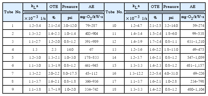
The table 1 summarized the volumetric mass transfer coefficient (kLa) with the gas flow rate for different flexible aeration tube diffusers operating within tap water. No matter what the gas diffusers are, the kLa coefficient increase with the gas flow rate from 1.2 × 10⁻³ to 4.0 × 10⁻³ 1/s for a gas flow rate varying between 1 and 4 L/min. Except the tube No. 16, the highest kLa values can be observed (1.2 × 10⁻² 1/s) but it needed the highest operational pressure (31.0 psi) that represented the highest power consumption was needed, in the same time. For the tube No. 4, it cannot be operated with 2 and 4 L/min of the air flow rate because it required too high of operational pressure that was over range of air pump and pressure gauge (over than 31 psi at 2 L/min of air flow rate). Even the air pump was fully turned on, but it can be operated just only 2 L/min. According to the over range of the operational pressure, the experiments for the tube No. 4 had to be stopped due to the safety concern.
Oxygen Transfer Performance of Flexible Aeration Diffuser Tube
In order to compare the performance of different gas diffusers more clearly, the aeration efficiency (AE) which is an oxygen transfer rate per power consumption should be taken into account. According to Fig. 3, the values of AE vary between 80 and 1,200 mg-O2/kW-s for a gas flow rate varying between 1 and 4 L/min. The highest AE or the highest energy performance was obtained with the tube No. 12 while the kLa and OTE were nearly the same value, then the tube No. 12 can be presented as the best flexible tube diffuser. Therefore, in order to provide a better understanding on the oxygen transfer performance from different gas diffusers, the related physical characteristics of different flexible aeration diffuser tubes used in this research will be well studied and presented in the next section.

Aeration efficiency of the different flexible tube diffusers.
5.2. Physical Characteristic of Flexible Aeration Diffuser Tube
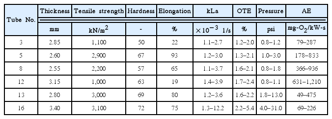
In this part, the 6 samples of the tube diffuser (No. 3, 5, 8, 12, 13, and 16) were chosen in order to analyze the related physical characteristics based on their oxygen transfer performance as previously presented. Table 2 shows the summary of the experimental results in terms of tube wall thickness, tensile strength, hardness and elongation. Note that the Vernier micrometer, Durometer and Tensile test were applied in order to measure the tube wall thickness, Tube hardness and Tube elasticity, respectively.
Physical Characteristic of Flexible Aeration Diffuser Tube
According to Table 2, it can be observed that the increase of tube wall thickness can increase the kLa coefficients: more non-uniform porous section presence in diffuser is probably related to the bubble generation phenomena (size and distribution). Moreover, the tube wall thickness can affect directly on the operational pressure (P), power consumption (PG), and thus the aeration efficiency (AE). The very high tensile strength and elongation obtained with several diffusers (No. 5, 13, and 16), should relate to elasticity behavior of diffuser tube in this study. These parameters increases the operational pressure due to the elasticity (P0) that cause the friction on orifice opening mechanism for bubble generation, and thus the operational pressure measured experimentally as shown in Fig. 4.
Operational pressure versus gas flow rate for different flexible aeration diffuser tubes.
It can be concluded that the physical tube characteristics can be applied in order to describe the oxygen transfer mechanism and thus to select the suitable flexible aeration diffuser tube. For example, the highest kLa coefficient and lowest AE obtained with the tube No. 16 should be corresponded to their wall thickness and tensile strength. Considering to the tube hardness obtained in this study, the results obtained with different diffusers were close to 50 and 72: this can possibly affect on the flexible tube structure and orifice size modification at different gas flow rate. From this study, due to the values of kLa and OTE, the tube No. 12 should be, therefore, applied in order to produce the practical flexible aeration diffuser tube. Figure 5 presents the image analysis results of the tube No. 12. Note that the tube wall and section were obtained with the 50× Scanning Electron Microscopes (SEMs). The orifice size and modification was measure by 4× Microscope.
Image analysis results of flexible tube No. 12. (a) Flexible tube surface; (b) Section view of tube; (c) Orifice diameter.
According to Fig. 5, it can be observed that high amount of porous presence on the tube wall (a): this can serve as the diffuser orifice for bubble generation. Moreover, non-uniform porous and channeling were found in the tube section (b). The average orifice diameter was equal to 0.19 mm and independent to the gas flow rate (1–4 L/min): the characteristic of tube hardness should be responsible for these results. In next section, the bubble hydrodynamic parameters (bubble size, bubble formation frequency and their rising velocity) will be determined, as well as, the interfacial area (a) in order to describe the oxygen transfer mechanism related to the generated bubbles from different flexible aeration diffuser tubes and to confirm the selection of suitable gas diffuser.
5.3. Bubble Hydrodynamic Parameters and Interfacial Area
According to the best flexible tube diffuser, tube No. 12 was chosen to analyze the detached bubble diameter (dB) and their rising velocity (UB) in the function of the gas flow rate as shown in the Fig. 6.

Interfacial area of flexible tube No. 12.
As shown in table 3, the generated bubble size was roughly constant for whatever the air flow rate: these results relate to the rigid orifice behavior: the bubble size was controlled by the fixed orifice size (≈ 0.19 mm for tube No. 12) [4]. Therefore, it can be stated that the tube hardness characteristics can play the important role on diffuser behavior (flexible or rigid), and thus on the variation of bubble size. For a given gas flow rate, the order is found: the bubble diameter of the tube No. 16 was larger than the tube No. 12 and the tube No. 3, respectively. These results correspond to the tube elasticity characteristic as presented in Table 2. This can be explained that the increase in the bubble diameter with the elasticity is characteristic of flexible membrane sparger [2]. This is caused by the fact that with higher elasticity, a larger hole (orifice) in the material can bulge and yield the higher bubble size. However, at higher gas flow rate, the bubble size obtained with the tube No. 3 (2.45 mm at 4 L/min of air flow rate) was greater than those obtained with the other diffusers. These results confirm the importance of tube hardness characteristic on the bubble generation phenomena due to the orifice size modification. It can be also noted that the generated bubble sizes obtained in this section were also controlled by the static surface tension (σTap water = 72.2 mN/m) from the same liquid phase used in this study.
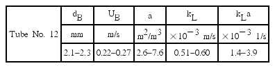
Bubble Hydrodynamic Parameters of Flexible Tube No. 12
For the rising bubble velocities obtained experimentally vary between 0.22–0.27 m/s. It can be observed that the UB values seem to be increased with the gas flow rate. Moreover, the UB values are closed to those given by the diagram of Grace & Wairegi [9]. By using the experimental results of the bubble diameter (dB) and the bubble rising velocity (UB), the calculated bubble formation frequencies (fB) related to the gas flow rates can be calculated. The interfacial area increases linearly with the gas flow rate. The a-area vary between 4.7 and 13.8 m2/m3 whereas the gas flow rates change between 1 and 4 L/min. Theoretically, the values are directly linked to bubble diameter, bubble rising velocity and static surface tension of liquid phases under test. The effects of physical characteristic on the bubble formation phenomenon and on the interfacial area being clearly proved, their consequences on the liquid-side mass transfer coefficient (kL) have to be evaluated now: this is the aim of the next section.
5.4. Liquid-Side Mass Transfer Coefficient (kL)
As shown in the table 3, the liquid-side mass transfer coefficient (kL) following by the gas flow rate between 5.10 × 10⁻⁴ and 6.0 × 10⁻⁴ m/s when gas flow rates varying between 1 and 4 L/min. Whatever the gas flow rates, the kL values remain roughly constant for each diffuser. These results conform to those of Calderbank and Mooyong [10]: the authors have shown that the kL values are constant for bubbles having diameters greater than 2–3 mm behaving usually like fluid particles with a mobile surface. Note that the bubble sizes generated in this study were controlled by tube physical characteristic and greater than 2 mm (Fig. 8). Moreover, the lowest and highest kL coefficients were obtained with the tube No. 3 and tube No. 16, respectively. Due to the existing kL model [8, 12], the experimental kL values vary between the two equations:

Comparison of kLa coefficient and pressure of the flexible tube No. 12 in the pilot-scale. (a) Comparison of the kLa coefficient; (b) Comparison of the pressure.
where h is the bubble height close to its diameter at low gas flow rates (Fig. 6). Re the bubble Reynolds number (
5.5. Installation Test in Pilot-Scale Experiment
After the flexible tube No. 12 was presented as the best tube with the optimum physical properties, the pilot-scale experiment was set up in 2,000 L of aeration tank to validate its performance and find out the best installation pattern. The 7.5 m of tube was assembled and arranged at the bottom of the tank with the same length of tube per surface area of the aeration tank as conducted in the lab-scale, as shown in Fig. 7. The best installation pattern was the pattern No. 2 which separated the tube into 16 branches that can cover overall area of the aeration tank, and the shortest tube for each branch produced the lowest operational pressure, comparing to the others pattern. The kLa of the pattern No. 2 slightly increased from 2.4 × 10⁻³ to 4.9 × 10⁻³ L/s with the air flow rate varying between 60–100 L/min. And the operational pressure was the lowest around 3.5–5.5 psi, as shown in fig. 8. Considering to the length of the tube per branch, the order was found that pattern 3 > pattern 1 > pattern 2, which were 7.5, 3.75, and 0.47, respectively. This result corresponds to the operational pressure that relate to the power consumption. So, the pattern No. 2 is the suitable installation in the pilot-scale by the lowest operational pressure or the highest aeration efficiency.
Experimental set up and installation pattern in the pilot-scale. (a) 2,000 L of aeration tank; (b) Installation pattern No.1; (c) Installation pattern No.2; (d) Installation pattern No.3.
5.6. Residence Time Distribution Study (RTD)
The residence time distribution (RTD) and Peclet number (Pe) were analyzed in this aeration tank, followed to Moustiri et al., 2001 [12], to study water flow pattern or mixing level within the tank. The aeration tank was operated as a CSTR reactor together with aeration, at 45 L/min of continuous water flow, 70 L/min of the air flow rate, and used NaOH solution as a tracer pulse that was monitored in form of conductivity. It was found that all of the installation patterns had the same trend of the conductivity which increased immediately when the NaOH was dosed, after that it was slightly decreased with time, after that the result was calculated in term of the exit age (E(t)) in the function of time as shown in fig. 9. Then the trend of E(t) was analyzed in form of average residence time (ART) which it was around 49.4–50.5 min, comparing to 56.3 min of the designed residence time, this result represented the short circuit flow was occurred during the operation period. For the peclet number, all of the patterns had nearly the same Pe values which closed to zero (in the scale of 0–1), as shown in table 4. The result showed that all of the installation patterns can lead the completely mixed flow in the aeration tank which it was expected for the oxygen transfer and distribution during the aeration process by using the flexible tube as a diffused aerator.
Comparison of conductivity with time.
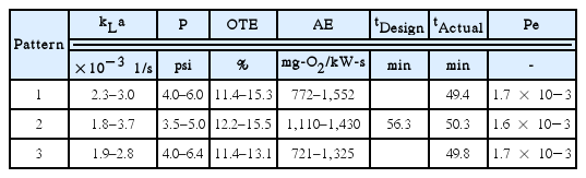
Residence Time Distribution Study of Flexible Tube No. 12 in the Installation Test
5.7. Theoretical Prediction Model for Oxygen Transfer Parameters
According to Painmanakul et al. 2009 [13] who proposed the suitable theoretical prediction model for predicting the bubble hydrodynamic and mass transfer parameters by predicting the kL coefficient and interfacial area. Then the kLa can be obtained as a product of the two parameters, by following equations,
After the prediction models were validated together with correction factors, it was found that the predicted results were closed to the experimental results with the error less than 30% even in the pilot-scale, as shown in fig. 10.
Comparison of the experimental and predicted kLa coefficient of flexible tube No. 12.
Then, these prediction methods can be applied in order to predict the kLa coefficient as a primary data for aeration process design. However, it should be studied for further in the real aerated water and large scale of the aeration tank, to improve the predictable accuracies. Moreover, the various types of aerator and operating conditions should be applied for validating the proposed kLa prediction method.
6. Conclusions
This study has shown that the physical diffuser tube properties play the important role on the power consumption, operating cost, bubble hydrodynamic parameters and thus oxygen transfer efficiency. The related results have shown that;
The volumetric mass transfer coefficient increases with the gas flow rates whatever the gas diffusers. The highest kLa values can be obtained with the tube No. 16;
The aeration efficiency (AE) should be considered in order to compare the different gas diffusers and select the suitable design and production;
The physical diffuser properties (tube wall thickness, tensile strength, orifice size, hardness and elongation) have been proven to be the key factor that controls the oxygen transfer performance;
The effects of physical diffuser properties (tube hardness and elongation) on the bubble formation phenomenon, orifice size and the interfacial area were clearly proved;
It is not necessary to generate too much fine bubbles to increase the interfacial area: this relates to high power consumption and the great decrease of the kL coefficient.
Due to the values of kLa, OTE, a and kL obtained in this study, the physical diffuser properties associated with the tube No. 12 should be applied in order to produce the practical flexible aeration diffuser tube.
In the future, the effect of different contaminants presence in liquid phase should be analyzed. The theoretical prediction models should be proposed for the bubble hydrodynamic and mass transfer parameters prediction, in the real aerated water and large scale of the aeration tank. Moreover, it is evident that the results observed in our small bubble column volume have to be validated into a tall bubble column and at higher superficial velocities.
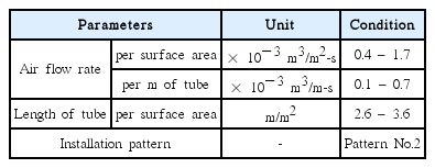
The Recommended Operational Condition for the Flexible Aeration Diffuser Tube
Acknowledgements
This work has the financial support from the Ratchadapisek Sompoch Endowment Fund (2016), Chulalongkorn University (Project Number CU-59-022-FW) and research funding of Faculty of Engineering, Chulalongkorn University. The authors would like to acknowledge the Graduate school of Chulalongkorn University, Center of Excellence for Environmental and Hazardous Waste Management (EHWM) of Chulalongkorn University for additional financial and technical support, as well as, CHAREON PHATARA PANICH CO., LTD. for materials supply.