Optimization of coagulation conditions for pretreatment of microfiltration process using response surface methodology
Article information
Abstract
The application of coagulation for feed water pretreatment prior to microfiltration (MF) process has been widely adopted to alleviate fouling due to particles and organic matters in feed water. However, the efficiency of coagulation pretreatment for MF is sensitive to its operation conditions such as pH and coagulant dose. Moreover, the optimum coagulation condition for MF process is different from that for rapid sand filtration in conventional drinking water treatment. In this study, the use of response surface methodology (RSM) was attempted to determine coagulation conditions optimized for pretreatment of MF. The center-united experimental design was used to quantify the effects of coagulant dose and pH on the control of fouling control as well as the removal organic matters. A MF membrane (SDI Samsung, Korea) made of polyvinylidene fluoride (PVDF) was used for the filtration experiments. Poly aluminum chloride (PAC) was used as the coagulant and a series of jar tests were conducted under various conditions. The flux was 90 L/m2-h and the fouling rate were calculated in each condition. As a result of this study, an empirical model was derived to explore the optimized conditions for coagulant dose and pH for minimization of the fouling rate. This model also allowed the prediction of the efficiency of the coagulation efficiency. The experimental results were in good agreement with the predictions, suggesting that RSM has potential as a practical method for modeling the coagulation pretreatment for MF.
1. Introduction
Microfiltration (MF) and ultrafiltration (UF), which are low-pressure membrane filtration processes, has been adopted to replace conventional methods for potable water treatment [1, 2]. The application of microfiltration and ultrafiltration processes for water treatment has rapidly increased since the mid-1990s [3, 4]. This is attributed to their ability to satisfy stringent regulatory requirements for not only turbidity but also pathogens such as Giardia cysts and Cryptosporidium oocysts. Moreover, continuous advances in membrane technologies have lowered the costs for membrane filtration, which is now economically competitive with conventional sand filtration [4].
However, MF and UF systems have inevitable problems caused by membrane fouling [5, 6]. Membrane fouling is defined as deposition of solute or particles on a membrane surface or inside membrane pores, which lead to reduce the membrane’s original permeability. Membrane fouling results in an increase in trans-membrane pressure to produce water and thus increases water production cost [7, 8]. Accordingly, many researchers and operators have studied pretreatment technologies to mitigate membrane fouling, including dissolved air floatation, coagulation, sedimentation, and sand filtration [9–15].
Among these pretreatment techniques, coagulation is the most popular process to control membrane fouling due to colloids and organic matters in the feed water. Using coagulation, the colloidal particles aggregate each other to form chemical flocs. The flocs have lower hydraulic resistance than individual particles, leading to reduced membrane fouling. Since this technique is inexpensive and effective, many water treatment plants use a combination of coagulation with membrane filtration [16].
In conventional water treatment, coagulant dose is determined by conducting jar tests. However, this jar test is only useful to examine the settling efficiency of chemical flocs. In membrane systems, however, it is not necessary to apply sedimentation after coagulation. Thus, the jar test is not a suitable method to determine the optimum coagulation conditions. So, a new technique to optimize coagulation pretreatment for membrane filtration should be developed.
In this context, the objective of this study was to develop a method to explore the optimized coagulation conditions for MF feed pretreatment. A response surface methodology was adopted for systematic optimization of the coagulation conditions. This technique allows the derivation of empirical equation for predicting the effectiveness of coagulation process [17]. Accordingly, it can be also used for system control and may have a lot of applications.
2. Materials and Methods
2.1. Feed Water
Feed water was sampled from Han-river in Korea. This is a major water supply to Seoul metropolitan area. Table 1 summarizes the water quality parameters for the feed water.

The Water Quality of Han Liver as Feed Raw Water
2.2. Coagulation Conditions
Poly-aluminum chloride (PAC as 17% Al2O3) was added into the feed water for the pretreatment of MF process. A jar-tester (YUYU Scientific M.F.G, Korea) was used for coagulation treatment. The working volume of each feed tank was 2 L. Details in the experimental conditions are provided in Table 2.
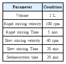
The Operation Conditions of Jar-tester for Coagulation
2.3. Membrane Filtration
The membrane filtration tests were conducted using a laboratory-scale equipment. This allows the use of maximum 15ea of MF submerged hollow fibers to simultaneously evaluate their performances by measuring transmembrane pressure (TMP). The constant flux mode was adopted to monitor the changes in TMP with time. Accordingly, this experiment was capable of comparing the membrane fouling rate before and after coagulation. A multi-channel cartridge peristaltic pump (EW-07551-00; Cole-Parmer, USA) was used for membrane filtration. The TMP was continuously recorded using pressure transmitters (ISE40A-01-R; SMC, Japan) connected to a data logger (usb-6008; NI, USA). Then, the results were used for further analysis of the fouling rate.
A schematic diagram of the laboratory-scale equipment was illustrated in Fig 1. Each membrane was vertically placed into each water tank of 1L volume. The material of the MF membrane used in this study was polyvinylidene fluoride (PVDF). The manufacturer of the membrane was Samsung SDI in South Korea. The membrane had a nominal pore size of 0.03 μm, an internal diameter of 0.8 mm and an external diameter of 2.1 mm. The detailed information of membrane used in the experiment was given in Table 3. The water temperature was marinated at 20°C and the flux was fixed at 90 L/m2-h.

Schematic diagram of a device for MF membrane performance.

Specification of the MF Hollow Fiber Membrane
2.4. Water Quality Measurement
The UV absorbance at the wavelength of 254 nm was determined using a spectrophotometer (DR/4000U; HACH, USA) and the turbidity was measured using a turbidity meter (Turb 430 IR; WTW, Germany).
2.5 Theoretical Fundamentals
A simplified filtration model based on the resistance-in-series model was used to examine the fouling rates of dead-end microfiltration. Among various fouling mechanisms, only model equations for cake filtration mechanism was adopted here. According to this approach, the Darcy’s law can be used [18]:
where J is the flux of the permeate; ΔP is the transmembrane pressure; η is the water viscosity; Rm is the intrinsic hydraulic resistance; and Rc is the hydraulic resistance for the cake layer formed on the membrane surface. The Rc is proportional to the ratio of cake mass (mc) to membrane area (Am).
where α is the specific resistance of the cake layer. Then, the following equation can be derived:
where t is the time for membrane filtration and cf is the effective concentration of the foulants. It should be mentioned here that cf and cb (the bulk concentration of foulants) are different due to the existence of critical flux. Finally, ΔP can be expressed as:
Here, θ is the fouling rate, which can be experimentally obtained from the slope of the graph for t and ΔP.
Eq. (4) indicates that θ is linearly proportional to J2. Accordingly, θ increases with an increase in J even if cf and α are constant. In other words, θ is affected not only by the feed water characteristics (ηαcf) but also the operation condition of the membrane (J). Thus, the normalized fouling rate, θ/J2, was used to quantify the fouling potential of the feed water instead of θ.
2.6. Response Surface Method
Response surface methodology (RSM) is one of the techniques to explore the correlations between independent variables and dependent variables. The first goal of RSM is to determine the optimum conditions for the response using statistical approaches. The second goal is to understand how the response changes with an adjustment of the design variables. Thus, the application of RSM focuses on the reduction in the cost of expensive analysis methods and their associated numerical errors [19]. The design of experiment such as a central composite design (CCD) may be used to obtain second-degree polynomial models for approximation of the experimental results. Then, this model can be used to optimize the conditions for a target variable [20].
2.6.1. Experimental design
In this study, CCD was used with two variables and five levels (i.e., −1.414, −1, 0, 1 and 1.414). The concentration of coagulant (X1) and pH (X2) were selected as the independent variables. The normalized fouling rate (Y1), turbidity (Y2), and UV-254 (Y3) were selected as the responses. Each represents the fouling potential, particle concentration, and humic-like organic concentration for the pretreated water, respectively. The measurement for the turbidity and UV-254 was triplicated. Table 4 summarizes our design of experiment.

The Central Composite Design and the Resulted Responses
2.6.2. Statistical analysis and regression analysis
A set of second order polynomial models were obtained using the experimental results analyzed by Minitab® 16.2.0 (Minitab, USA). The general form of the equations is given by:
where Yk is the responses of the independent variable; βk0, βki, βkii and βkij are the coefficients; and Xi is the independent variables. The suitability of the equations is examined based on R2 value and the lack-of-fit (LOF).
3. Results and Discussion
3.1. Analysis of Membrane Fouling Based on the Response Surface Method
According to the design of experiment listed in Table 4, RSM was applied to determine the optimum coagulation conditions for pretreatment of MF. As a result of the RSM analysis, two model equations were obtained and their statistical significance was examined by the analysis of variance (ANOVA). Table 5 shows the regression coefficients for the models for the normalized fouling rate (Y1), turbidity (Y2), and UV-254 (Y3). The terms that are not statistically significant (p > 0.05) were omitted from the regression equation. The final forms are given by:
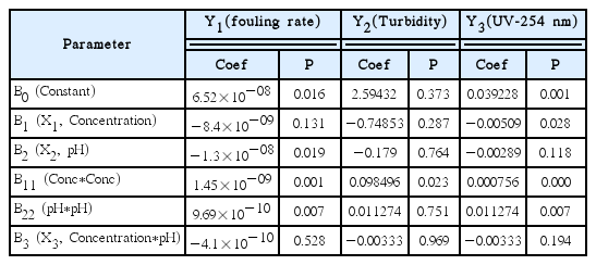
Coefficients of the Fitted Polynomial Models for Responses
According to the results of ANOVA, Y1 (fouling rate) and Y3 (UV-254 nm) are dependent on X1 (coagulant concentration) and X2 (pH). However, Y2 (turbidity) seems to depend only on X2 (pH). This is probably because the turbidity was not sensitive to the operation conditions under the coagulation conditions considered in these experiments. In Eq. (6) and Eq. (8), the quadratic terms of X1 and X2 are significant. On the other hand, in Eq. (7), the quadratic term of X2 is significant. In Eq. (8), the quadratic term of X2 is significant. All the interaction terms were not included due to low significance.
The results of ANOVA are shown in Table 6. The R2 for the three equations were 90.21, 68.63 and 98.10, respectively. This suggests that the regression is statistically significant. The lack-of-fit results also indicate that the regression is reasonable. It is evident from these results that the model equations represents the dependence of responses on the independent variable.
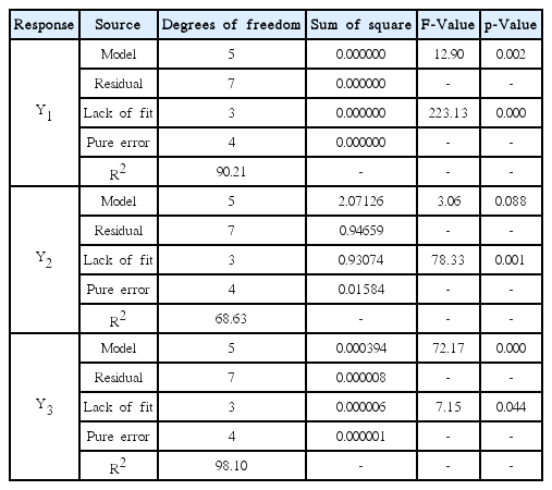
Analysis of Variance (ANOVA) for the Polynomial Models
3.2. Influence and Interaction of Independent Variables
The influences of the independent variables on the responses are presented as response surfaces in Fig 2 and 3. The interactions between the variables are also shown in these plots.

Response surface plots for coagulation conditions and efficiencies.
As shown in Fig 2, they have similar graph form at the same condition. Three graphs indicated that it becomes better with high coagulant doses from 4 to 5 mg/L and pH 7.5. This result implies that high coagulant dose and neutral pH results in low fouling rate and high water quality.
The contour and surface plots are illustrated in Fig 3. The fouling rate and UV-254 are more strongly dependent on pH range. On the other hand, pH showed little effect on the turbidity removal. These results imply that there are non-linear interactions among the independent variables. Accordingly, the optimum conditions cannot be determined without the use of the RSM analysis.
The overlaid contour plot obtained after RSM analysis was illustrated in Fig 4(a). The white area means the point meeting three requirements at the same time. The three requirements were ranged from 4.9×10⁻¹⁰ to 1.1×10⁻⁹ in fouling rate; from 0.35 to 0.55 NTU in turbidity; from 0.018 to 0.022 ABS/cm in UV-254 nm. The results indicate that the modeling results match the experimental data well. Based on the results of RSM analysis, the desired operation conditions can be obtained using the response optimizer. Fig shows the optimum conditions for fouling rate, turbidity, and UV-254 nm. According to this result, the optimum coagulant dose and pH are 3 and 7.5, respectively. Under this condition, fouling rate, turbidity and UV-254 nm are 7.7×10⁻¹⁰, 0.5 NTU and 0.02 ABS/cm respectively.

(a) Contour plot and (b) Response optimizer of the influences of independent variables for responses.
4. Conclusions
This study was intended to apply RSM to optimize the coagulation conditions for MF pretreatment. The following conclusions can be drawn:
Using a simple model, the normalized fouling rates were experimentally obtained depending on the coagulation conditions. The model was useful to analyze the experimental results from a laboratory-scale MF equipment.
RSM was introduced to examine coagulation efficiency as a function of coagulant does and pH. This technique was found to be useful to examine the interactions between the independent and dependent variables.
Compared with the RSM models for coagulant dose and pH, the model equation for turbidity was less reliable. This was attributed to the wider error range of the turbidity measurement data.
Using the RSM equations, the optimum coagulation condition was estimated: The coagulant dose ranges from 3 mg/L to 5 mg/L and the pH ranges from 7 to 8. It is expected that this approach has potential for process control of pilot or full-scale membrane plant.
Acknowledgements
This research was supported by the Korea Ministry of Environment as “The Eco-Innovation project (Global Top project)”. (GT-SWS-11-02-007-9 and GT-SWS-11-01-002-0)