

1. Introduction
The first sewage treatment plant of Korea, Jungrang Sewage Treatment plant, was introduced in 1976, which was late compared to the installments of other city infrastructures. However, according to the data in 2009, there were 438 sewage treatment plants treating over 500 m3 per day with the total facility capacity of 24,735,000 m3 per day. Also, there were 2,332 sewage treatment plants treating below 500 m3 per day with the total facility capacity of 171,000 m3 per day; and consequently, the percent of population being supplied with sewage was 89.4%, which was not lacking compared to other developed countries in the world [1]. Also, a vast improvement has been made in terms of sewage treatment processes compared to the days when there was only the activated sludge process, which targeted organic matters; now, there are advanced sewage treatment processes that target various nutrients and poisonous substances. However, there is still huge room for improvement in terms of the operation and management technology of sewage treatment plants.
Operating a sewage treatment plant involves biological processes with complex reactions, which make it difficult to understand the behavior of the processes. Therefore, it requires a lot of analysis in order to fully understand the processing conditions and behaviors. Consequently, almost all of the operations within the sewage treatment plants rely heavily on experience. This is not desirable in terms of the automation of sewage treatment processes and reduction of personnel expenses. If a sewage treatment plant is operated based on the operator’s experience, it is very difficult to conserve the energy spent within the sewage treatment plant.
In 1987, the International Association on Water Pollution Research and Control (IAWPRC) introduced the ASM1 model based on the analysis of the sewage treatment process using mathematical models. The ASM1 model was followed up by ASM2, ASM2d, and ASM3. These models are rational models with excellent emulation abilities. There are commercial programs applying these models that are being developed and used. But the analysis for substance classification and the measurement of the parameters using these models is difficult. Therefore, it is difficult to predict and control the sewage treatment process using these models in real-time. To solve these problems, there are various researches going on, such as the Benchmark Simulation Model, ARIMA Model, Neural Network Model, Multi Objective Model, ASMs simplifications, etc. [2–10].
Therefore, a multiple regression model that predicts and controls the sewage treatment process was developed utilizing the actual operational data being analyzed on a daily basis at the sewage treatment plants in this study. Also, the operational parameter prioritization methods with respect to effluent quality standards were developed by analyzing the influence of each operational parameter based on the results from the model above.
2. Materials and Methods
2.1. Selected Sewage Treatment Plant
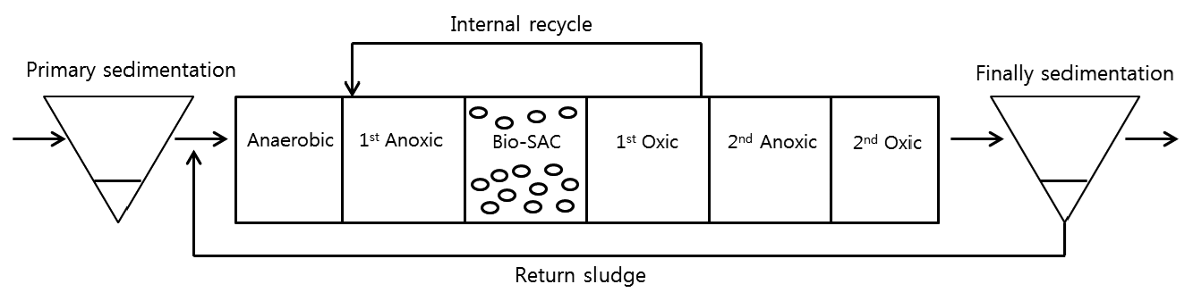
The sewage treatment plant within this study, the P sewage treatment plant (232,000 ton/day) uses the media process (Fig. 1). The bioreactor process was chosen for the model development process and we reviewed the process starting with the intake of the influent and ending up with the release of the effluent. All of the data used in this research are within the year 2012.
2.2. Multiple Regression Analysis
Multiple regression analysis is a statistical method that analyzes the relationship between the dependent variable (Y), and independent variables (X1, X2, X3, ...). Any variables leading to multicollinearity during the multiple regression analysis were eliminated from the model, and any outliers and influential observations were considered through residual analysis in the model.
Multiple regression analysis used the SAS 9.2 program (SAS Institute Inc., Cary, NC, USA) and the stepwise method was implemented as the variable selection method. The significance level for the model verification and variable selection through the variable selection method was set at 0.05.
There were a total of 32 variables for the multiple regression analysis. RO_COD (2nd settling tank effluent CODMn) and RO_TN (2nd settling tank effluent T-N) were set as dependent variables and the remaining 30 variables were set as independent variables (Table 1).
2.3. Analysis Method
In the multiple regression analysis, the model was developed using the data from January 2012 to October 2012 and the data from November 2012 to December 2012 were used to verify the accuracy of the model.
The studentized residual suggested by Belsley et al. [11] and the DFFITS were used to verify the outliers and influential observations in this study. The following conditions had to be established between the studentized residual and the DFFITS in order to determine whether they were outliers or influential observations [11–14].
Outliers criterion using the studentized residual:
Influential observations criterion using the DFFITS:
In this case, k is the number of independent variables and n is the number of samples.
For checking multicollinearity, the stepwise method was used to set a variable and the variable’s variance inflation factor (VIF) was calculated. If there was a variable greater than the VIF by 10 or more, it would be eliminated from the model development process after review and another variable would be selected by the stepwise method.
For verifying the accuracy, the following equation was used.
In this case, yi is the i-th observed value, ŷi is the i-th predicted value, and l is the total number of values in the prediction data.
Multiple regression analysis was carried out through 8 cases depending on the variable selection method, elimination of outliers and influential observations, and log conversions (Table 2). In cases 1 to 4, the stepwise method was implemented as the variable selection method for all variables, and from cases 4 to 8, variables that are capable of being operated and controlled at the sewage treatment plant (aerobic reactor DO, aerobic reactor MLSS, return sludge amount, excess sludge amount) were selected and they were all included in the model development, if the stepwise method was applied. Standardized regression coefficients were considered in order to compare the effects of each parameter through multiple regression analysis for each case.
3. Results and Discussion
After reviewing the multiple regression model based on two variables RO_COD (2nd settling tank effluent CODMn) and RO_TN (2nd settling tank effluent T-N), all values resulting from the F-test on each case were below 0.05, which is statistically significant.
3.1. RO_COD (2nd Settling Tank Effluent CODMn)
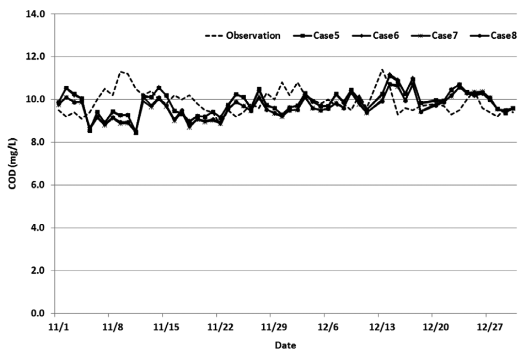
After performing multiple regression analysis through 8 different cases, it was discovered that the variance patterns of the actual values and the predicted values for every case were similar. Also after reviewing factors that could explain the actual values resulting from the multiple regression model, such as the coefficient of determination, accuracy of prediction, and root mean squared error, all 8 cases displayed similar values (Table 3). The graphs comparing the observed values and predicted values for each case are show in Figs. 2 and 3.
3.2. RO_TN (2nd Settling Tank Effluent T-N)
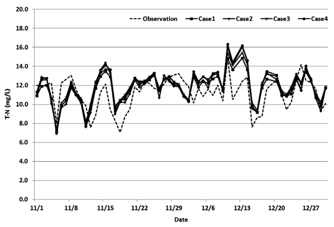
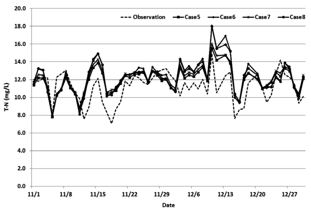
After performing multiple regression analysis through 8 different cases, it was discovered that the variance patterns of the actual values and the predicted values for every case were similar. Also, after reviewing factors which could explain the actual values resulting from the multiple regression model, such as the coefficient of determination, accuracy of prediction, and root mean squared error, all 8 cases displayed similar values (Table 4). The graphs comparing the actual values and predicted values for each case are shown in Figs. 4 and 5.
3.3. Selection of Multiple Regression Model
The regression model for each dependent variable was selected after reviewing the R2 (coefficient of determination) value, accuracy of prediction, root mean squared error, and variance pattern’s predictabilities.
In the case of dependent variable RO_COD (2nd settling tank effluent CODMn), case 4, which scored the highest in terms of R2 (coefficient of determination) value and accuracy of prediction, was selected and a regression model could be constructed based on the regression coefficients of each independent variable (Table 5).
In the case of dependent variable RO_TN (2nd settling tank effluent T-N), case 1, which scored the highest in terms of root mean squared error and accuracy of prediction, was selected and a regression model could be constructed based on the regression coefficients of each independent variable (Table 6).
A multiple regression equation for each dependent variable could then be formulated using the regression coefficients in Tables 5 and 6 above, and a prediction model for water quality predictions could be developed for each dependent variable depending on the changes made to independent variables, using the multiple regression equation.
3.4. Reviewing the Influence of Operation Parameters
Standardized regression coefficients were considered in order to review the influence of the operation parameters based on the model selected for each dependent variable. As the absolute value of the standardized regression coefficient grew larger, the influence on the model became greater.
In case 4, which selected from the dependent variable of RO_COD (2nd settling tank effluent CODMn), the order of the highest standardized regression coefficient among 11 independent variables was OUTF, I_COD, AE_MLSS (Table 7).
In case 1, which selected from the dependent variable RO_TN (2nd settling tank effluent CODMn), the order of highest standardized regression coefficient among the 8 independent variables was AE_TEMP, I_TN, FM (Table 8).
Based on the results of the standardized regression coefficients for each dependent variable, an independent variable with the biggest influence on dependent variables could be selected. After reviewing the influence on dependent variables mentioned above, it was concluded that dependent variables COD and T-N could be controlled by controlling the operation parameter AE_MLSS (aerobic reactor MLSS) for COD and operation parameter FM (F/M ratio) for T-N at the sewage treatment plant from which data was collected to formulate the multiple regression equations.
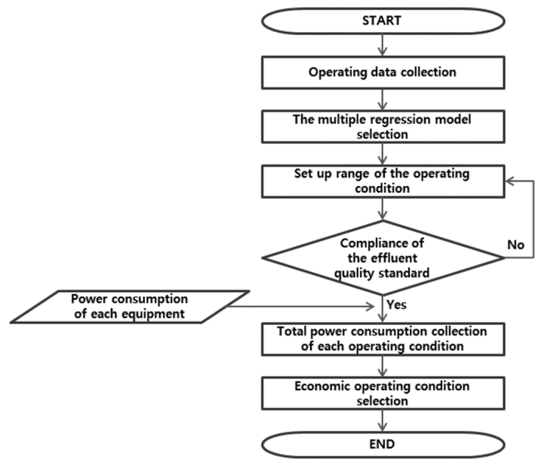
3.5. Reviewing the Economic Operation Condition of the Bioreactor
The method of process control utilizing the selected multiple regression model can provide the economic operation condition that saves energy without violating the effluent quality standards of CODMn and TN in terms of energy savings. In order to provide the economic operation condition, first, the power consumption of the equipment (blowers, internal return sludge pumps, excess sludge pumps, etc.) for operating the bioreactor should be reviewed. The economic operation condition can be provided by considering the effluent quality standards and the amount of power consumption (Fig. 6).
4. Conclusions
Using the prediction models for the 2nd settling tank effluent CODMn and T-N based on multiple regression analysis, it was shown that the accuracy of prediction came out to be above 0.93 and 0.84, respectively. Also, through this model, the variance pattern of the actual values was proven to have been predicted fairly well.
In the case of dependent variable RO_COD (2nd settling tank effluent CODMn), case 4 was selected, because it scored the highest in terms of R2 (coefficient of determination) value and accuracy of prediction; and in the case of dependent variable RO_TN (2nd settling tank effluent T-N), case 1, which scored the highest in terms of root mean squared error and accuracy of prediction, was selected.
Based on the results after reviewing the effectiveness of the operation parameters, the most effective operation parameter for controlling CODMn was AE_MLSS and F/M for controlling T-N.
The effectiveness of the operational parameters on the 2nd settling tank effluent CODMn and T-N were verified by reviewing the standardized regression coefficients of the multiple regression models constructed in this study. Predicting the concentration of CODMn and T-N in the 2nd settling tank effluent was possible by following the operation conditions using the selected multiple regression model. If the data on the energy spent on each operation parameter can be collected, then the operation parameter that conserves energy without violating the effluent quality standards of CODMn and TN can be determined using the regression model and the standardized regression coefficients. These results can provide appropriate operation guidelines to conserve energy to the operator at a sewage treatment plant that consumes a lot of energy.