The analysis of groundwater table variations in Sylhet region, Bangladesh

Md. Abu Zafor; Md. Jahir Bin Alam; Md. Azizur Rahman; Mohammad Nurul Amin

doi:10.4491/eer.2016.152

Environ Eng Res > Volume 22(4); 2017 > Article

Zafor, Alam, Rahman, and Amin: The analysis of groundwater table variations in Sylhet region, Bangladesh

Research Article

Environmental Engineering Research 2017; 22(4): 369-376.

Published online: May 1, 2017

DOI: https://doi.org/10.4491/eer.2016.152

The analysis of groundwater table variations in Sylhet region, Bangladesh

Md. Abu Zafor¹, Md. Jahir Bin Alam^2,^*, Md. Azizur Rahman^1,^*,^†, Mohammad Nurul Amin²

¹Department of Civil Engineering, Leading University, 5th floor, Rangmahal Tower Bandar Bazar, Sylhet-3100, Bangladesh

²Department of CEE, Shahjalal University of Science & Technology, Akhalia, Sylhet-3100, Bangladesh

^†Corresponding author: Email: azizraj0110@gmail.com, Tel: +88-0821-723625, Fax: +88-0821-720307

* These authors contributed equally to this work.

Received December 15, 2016 Accepted April 27, 2017

(open-access):

This is an Open Access article distributed under the terms of the Creative Commons Attribution Non-Commercial License (http://creativecommons.org/licenses/by-nc/3.0/) which permits unrestricted non-commercial use, distribution, and reproduction in any medium, provided the original work is properly cited.

Abstract

The trend analysis of the study was acquired by selecting multiyear monthly groundwater table data and monitors the wells in each sub-district under the study area. The intention of this research was to analyze the outcome of the non-parametric Mann-Kendall test at greater than the significance level which is 95% of groundwater level in Sylhet. The aptitude is effective at two conjunctures where the confidence bounds are 95% and it meets the estimate line of Sen’s. To calculate and assess the spatial differences in the inanition of groundwater table, geostatistical methods was applied based on data from 27 groundwater wells during the period from January 1975 to December 2011 which were obtained from a secondary source, Bangladesh Water Development Board. The geographic information system was used to assess the spatial change in order to find the level of groundwater. Cross-validation errors were found within an advisable level in estimating the groundwater depth with different interpolation models of ordinary kriging methods. Finally, surface maps were generated with the best-fitted model. The southeast region was found highly vulnerable from groundwater level point of view. Northern region was detected highest hazard prone area for diverge groundwater using kriging method.

Keywords: Geostatistical method, GIS, Kriging method, Mann-Kendall test, Sen’s method, Trend analysis

1. Introduction

Groundwater is considered as the most significant source of freshwater consumption in the world. Around 33% of world’s population relies on groundwater for the daily, industrial and agricultural purpose [1]. As world’s population is increasing day by day, the extraction of groundwater is also rising significantly. Groundwater extraction is the primary cause of increasing groundwater table in many areas [2–5]. Nowadays attenuation of groundwater level is ascertained as a global problem as it causes a couple of adverse effects including water pollution, saltwater intrusion, groundwater contamination, etc. [6–7]. Groundwater depletion has been estimated about 4,500 sq. km in total for the past century where maximum rates of depletion occurred in the period of 2000–2008 [8]. Groundwater consumption for irrigation purpose has risen significantly throughout the world, especially in South Asia, irrigation related to the producing rice directly rely on groundwater, and, Bangladesh is the world’s fourth-biggest rice producing country [9–10]. Recent studies showed that increasing trend in water table depth or declining trend in groundwater level which implies an unsuitable condition of groundwater in Bangladesh. In Dhaka city, dynamics of water table has been studied by Sarkar and Ali [11] and showed a steeply increasing trend in the water table. The trend analysis was carried out by nonparametric Mann-Kendall (MK) Test and Sen’s slope estimator. The similar procedure was also used in order to study the sustainability of groundwater resources by Ali et al. [12]. The study showed a similar output; rising trend in water table depth or declining trend in groundwater level in the North-Eastern region of Bangladesh. Also, the study revealed that if the similar trend continues, water table depth will increase significantly and will be double in most cases by 2060. Parametric regression approach has also been done in North-Western Bangladesh which displayed a drop in groundwater level in Barind area [13].

There are several statistical methods for trend analysis which vary from simple linear regression to more advanced parametric and non-parametric methods [14–15]. The most popular non-parametric method for analyzing the trend in the time series is the MK test [16–17]. MK test is a popular technique for analyzing the trends in climatic parameters, evaporation, reference evapotranspiration, stream flows and groundwater fluctuations [18–21]. The result was based on the MK trends analysis using the Sen’s template application [22]. In order to determine the magnitude of change per unit time of the trends detected, the Sen’s estimator was adopted [23]. This non-parametric aligned rank test was considered adequate because no underlying frequency distribution of data could be obtained. Salmi et al. [22] ruminate, in the cases where important significant trends are observed, statistical computation gives an eminent level of sharpness with narrow angles between the confidence lines. In this paper, the aptitude was substantial at two conjunctures where the confidence bounds were 95% and it met the Sen’s line of estimation.

Moreover, Sylhet district is the capital of Sylhet division and one of the most developed regions of Bangladesh. As most of the people primarily depend on groundwater, it is under tremendous pressure. Although recent studies have proved groundwater level is rapidly depleting over the last decade, no study was conducted for this area addressing trend and variation of groundwater level fluctuation. Therefore, it has been aimed in the study to display trend and spatial analysis of groundwater level fluctuation.

2. Materials and Methods

2.1. Study Area

Sylhet district is the center of the Sylhet division and consists of twelve sub-districts that lie on the banks of Surma river in north-east of Bangladesh with an area of 3,452.07 km². The average elevation of Sylhet district is 35 m. The climate of Sylhet is torrid monsoon with predominantly thermal and moist summer and a relatively cold winter. The annual average highest temperatures are 23°C (Aug-Oct) and the average lowest temperature is 7°C (Jan) because the settlement is in the monsoon climate zone. In between May and September, approximately 80% of the annual average precipitation (3,334 mm) occurs.

In the study area, there is limited information that is available or accessible in the aquifer systems. The main aquifer in the north-eastern region varies from semi-confined to confined types. A prospective aquifer in the north-eastern hills is the highly weathered alluvial sands of the Dupi Tila formation [24]. These sands are fine to medium grained and crop out in small hillocks in Sylhet and Moulvibazar districts and in some parts of Habiganj district. However, the permeability of these sands is lower than that of the alluvial deposits. The young gravelly sands also form a potential aquifer, although they are poorly sorted and contain large amounts of gravel and pebbles, making it difficult to use low-cost drilling techniques.

At present Groundwater is considered as the most important source of water supply in Bangladesh [25]. As a part of regular monitoring work by the Bangladesh Water Development Board (BWDB), the depths to groundwater are measured in piezometric observation wells situated in different parts of the study area. There are 27 observation wells in the study area which are considered in this study in order to determine the trend of groundwater depth. The observed variations are due to regional groundwater flow, head difference between the aquifers, and confining clay. Also, the population density of Sylhet district is 990/ km² which indicates a tremendous pressure as it is the major freshwater source.

2.2. Data Collection

There are 27 piezometric observation wells in Sylhet district. Data were collected from secondary sources. Data has been collected from BWDB. Monthly data for a period of 1975–2011 were obtained in the study for trend analysis. It was observed that groundwater table depth is increasing over the period. In 1975, the groundwater depth was found from 0.35–5.66 m where 22% increase in water table depth was observed by the end of 1985. Finally, in 2011, the depth to groundwater varied from 15–1.52 m which clearly indicates the groundwater level is declining over the period. In this study, trend analysis was conducted by collecting secondary data and using MK test and Sen’s estimator of the slope.

2.3. Methods of Analysis

The MK [16, 26] and Sen’s slope estimator test were employed for trend analysis and the slope of the trend line [23].

2.3.1. Mann-Kendall (MK) test

This method is significantly tested by applying time series data if there is a trend exists. The preliminary value of the MK statistic, S, is assumed to be 0 (for examples, no trend). S is incremented by 1 if the later time period of a date value is higher than another previous time period of the data value. Contrarily, S is incremented by 1, if the data value from an additional time period is lower than the previous time period. The procedure to compute this probability is stated in [27–28].

(1)

S = \sum_{k - 1}^{n} \sum_{j - k = 1}^{n} s i g n (X_{j} - K_{k})

Where,

\begin{array}{l} sign (x_{j} - x_{k}) = 1 if (x_{j} - x_{k}) > 0 \\ = 0 if (x_{j} - x_{k}) = 0 \\ = - 1 if (x_{j} - x_{k}) < 0 \end{array}

Where, S is eminent and equitable, it signifies that the trend is rising and a very small value suggests that the aptitude is declining. Nevertheless, it is necessary to compute this probability to statistically quantify the significance of the trend [27–28].

2.3.2. Sen’s estimator of slope

The method of calculating the Sen’s slope estimator requires a time series of equally spaced data. Sen’s method proceeds by calculating the slope as a change in measurement per change in time, as shown here in equation [23]:

(2)

Q = \frac{x_{j} - x_{k}}{j - k}

Where, Q is the slope between data points x_j and x_k, x_j is the data measurement at time j, x_k is the data measurement at time k and j is the time after time k.

2.4. Geostatistical Method

Geostatistics is a section of statistics which concentrate on spatial or spatiotemporal datasets. It is basically manifested to forecast probability distributions of ore grade mining operations. Nowadays it is applied in several systems including petroleum geology, hydrogeology, hydrology, meteorology, oceanography, geochemistry, geo-metallurgy, geography, forestry, environmental control, landscape ecology, soil science, and agriculture [29–30].

2.5. Spatial Prediction Method

2.5.1. Kriging

Kriging is a branch of geostatistical methods to interpolate the value of a random field (e.g., the elevation, z, of the landscape as a function of the geographic location) at unsighted whereabouts from the regard of its value at nearby locations [31]. This method is best suitable for normally distributed data. The data need to be resolved into normally distributed data using the transformation methods; if they are not normally distributed. The most usual transformation type is a logarithmic method because of its simplicity. The log transformation is as follows:

(3)

Y (s) = I n [Z (s)]

For Z(s) > 0 Where Z(s) is observed data, Y(s) is transformed normal data and in is the natural logarithm. Detailed discussions of kriging methods and their descriptions can be found in [30]. In kriging method, the most commonly used variogram models are spherical, exponential and Gaussian.

(4)

Exponential model: γ (h) = c_{0} + c_{1} {1 - exp (\frac{h}{a})}

(5)

Gaussian model: γ (h) = c_{0} + c_{1} {1 - exp (\frac{h^{2}}{a^{2}})}

(6)

\begin{array}{l} Spherical modle: γ (h) = [c_{0} + c_{1} {\frac{3 h}{2 a} - \frac{1}{2} {(\frac{h}{a})}^{3}}] for 0 < 0 < a \\ c_{0} + c_{1} for h \geq a \end{array}

Where, γ(h) is semi variance, h is lag, a is the range, C_o is Nugget variance, c₀ + c₁ = sill.

2.6. Generation of Best Fitted Models

The best-fitted models are generated by comparing the Mean Error (ME), Root Mean Square Error (RMSE), Average Standard Error (ASE) and Root Mean Square Standardized Effect (RMSSE). For the best prediction, the models must satisfy the following criteria [32].

The ME should be zero.
RMSE and ASE should be small as possible.
RMSSE should be close to 1.

For comparison of these models and data transformation, the following formula is used.

2.6.1. Root Mean Square Error (RMSE)

It is probably the most easily interpreted statistic since it has the same units as the parameter estimated. The RMSE is thus the difference, on average, of an observed data and the estimated data.

(7)

R M S E = \sqrt{\frac{1}{n} \sum_{i = 1}^{n} {[\tilde{Z} (X_{i}) - Z (X i)]}^{2}}

2.6.2. Mean Square Error (MSE)

For every data point, take the difference of the observed to the corresponding estimated values, and square the values. Then add up all those values for all data points, and divide by the number of points. The squaring is done so negative values do not cancel positive values. Smaller MSE indicates a better prediction of the data. The MSE has the units squared of the parameter estimated [33].

(8)

M S E = \frac{1}{n} \sum_{i = 1}^{n} [\tilde{Z} (X_{i}) - Z (X i)] / {\tilde{σ}}^{2} (X_{i})

2.6.3. Root Mean Square Standardized Effect (RMSSE)

This standardized measure of effect size is used in the analysis of Variance to characterize the overall level of population effects. It is the square root of the sum of squared standardized effects divided by the number of degrees of freedom for the effect [33].

(9)

R M S S E = \sqrt{\frac{1}{n} \sum_{i = 1}^{n} {[{\tilde{Z} (X i) - Z (X i)} / {\tilde{σ}}^{2} (X i)]}^{2}}

Where, σ̃2 (X_i) is the Kriging variance for location X_i. So, using ordinary kriging method each groundwater quality parameters can be generated.

3. Results and Discussion

Below Table 1 and Table 2 are provided in order to display cross-validation results and trend analysis of groundwater level in Sylhet district.

3.1. Result of Mann-Kendall Test and Sen’s Estimator of Slope

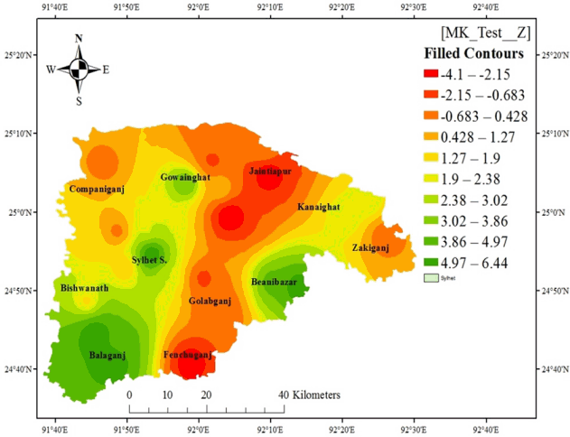
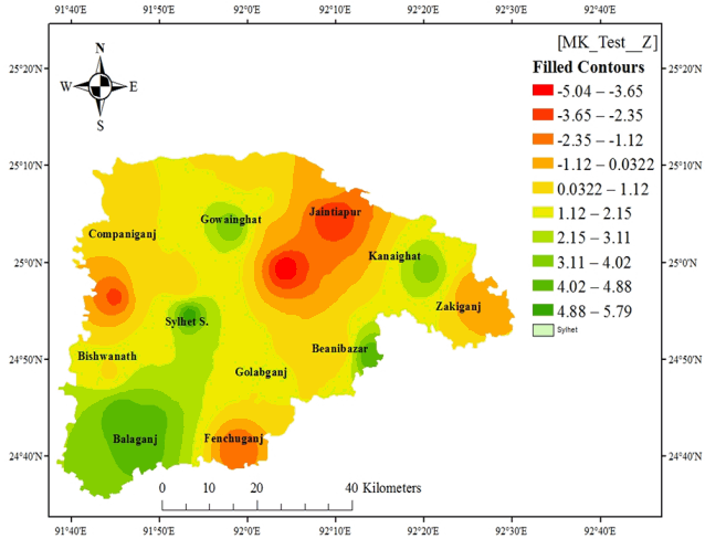
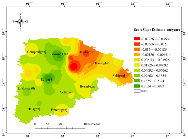
Variation in Groundwater Level Trends in some selected stations in Sylhet district. The results for groundwater level trend analysis are presented in Table 2 of the twenty-seven stations in the Sylhet District, thirteen stations had a significant trend at greater than 95% with test statistic Z ranging from −0.50 to 6.85. The trend is said to be decreasing if Z is negative and the computed probability is greater than the level of significance and increasing if Z is positive and the computed probability is greater than the level of significance. If the computed probability is less than the level of significance, there is no trend. From Table 2, it is evident that some of the stations in the Sylhet districts show no significant trend. However, Balaganj (GT9108002) show a very pronounced positive trend (increasing groundwater table depth) at Z equals to 6.85. Gowainghat and Jaintapur show relatively weaker negative trends at −3.53 and −1.65, respectively. Although there are many stations in Table 2 that showed relatively large upwards trends (increasing water table depth), only four are statistically significant. These Balaganj (GT9108001) (0.062 m/y), Balaganj (GT9108002) (0.063 m/y), Bishwhanath (GT9120006) (0.041 m/y), Golabganj (GT9138010) (0.088 m/y), Gowainghat (GT9141015) (0.0250 m/y).

Kanaighat (GT9159018) (0.023 m/y), Sylhet Sadar (GT9162021) (0.050 m/y), Sylhet Sadar (GT9162022) (0.068 m/y), (0.041 m/y), and Sylhet Sadar (GT9162026) (0.359 m/y). The magnitude of Sen’s slope estimate is shown in the bracket for each station. There are a few stations which showed a statistically significant downward trend. In Fig. 4 twenty-seven stations with statistical significant trend are presented.

Below Figs. 5 –7 display the rainfall trend (MK-Z test) for three periods of time, post-monsoon, rainy and winter, respectively.

Seasonal and annual trends for the period 2001–2012 is provided below in Fig. 8 that shows Sen’s slopes estimated in seasonal and annual time scales. The median of slopes in winter is lower compared with the other seasons. As expected, rainfall trends show large variability in magnitude and direction of the trend from one station to another. All the stations have a positive value of the Sen’s estimator for the post monsoon and summer seasons. As expected, rainfall trends show large variability in magnitude and direction of the trend from one station to another. All the stations have a positive value of the Sen’s estimator for the summer season.

Figs. 9 –11 explain the Sen’s slope variations in rainfall trends in pre-monsoon, rainy and winter.

4. Conclusions

By applying trend detection on homogenous zones groundwater level data (below PWD datum) in Sylhet district in Bangladesh, has resulted in identifying some significant trends. The study also represents the spatiotemporal variation of groundwater level in the study area. The direction of groundwater level trend was, in general, downward (i.e. groundwater table was upward) and statically significant across the study area. More than half of the stations that have shown highly significant trends, Sen.’s slope estimates varied between 0.359 and 0.023 mm/y, indicating groundwater level is lowering day by day. There were a few stations which reported a negative Sen’s estimator value in the whole of stations. Generally, a significant positive trend was observed to start in the mid-1975s in almost all the zones. These results demonstrate the impacts of anthropogenic developments in the study.

This research has clearly demonstrated that climate studies focusing on localized areas are possible and important since local-scale climate has direct relevance to large populations dependent on subsistence agriculture. A continuous decrease in groundwater level can be explained by the lack of strong local influences on rainfall formation like vegetation on mountains, also, increase in population that use more land for agriculture and settlement (urban sprawling). Moreover, Climate change effects at global to local scale might also be playing a role. Another concluding remark is that; continuous significant decline (at the > 95% level) was observed in the groundwater level. The scarcity of groundwater can be explained by the over-exploitation of groundwater resources for irrigation and domestic purpose, also, lacks of surface water is responsible for the growing demand of groundwater. The study suggests proper management so as to increase groundwater recharge and to find other alternative water resources in order to fulfill the water demand. However, if over-exploitation of forests will be avoided; for example, through assistance to meet communities’ basic needs within come generation opportunities, the vegetative cover can be restored. Poverty mitigation measures can include planting trees (for their products and services) in major a forestation schemes, woodlots, linear plantations, windbreaks, and agroforestry.

Acknowledgments

I wish expressing my profound thanks and sincerest appreciation to Bangladesh Water Development Board (BWDB) for providing and allowing the necessary data related to the research work.

References

1. Ahmadian M, Chavoshian M. Spatial variability zonation of groundwater-table by use geo-statistical methods in central region of Hamadan Province. Ann Biol Res. 2012;3:5304–5312.

2. Shamsudduha M, Chandler R, Taylor R, Ahmed K. Recent trends in groundwater levels in a highly seasonal hydrological system: The Ganges-Brahmaputra-Meghna Delta. Hydrol Earth Syst Sci. 2009;13:2373–2385.

3. Phien-wej N, Giao P, Nutalaya P. Land subsidence in Bangkok, Thailand. Eng Geol. 2006;82:187–201.

4. Bui D, Kawamura A, Tong T, Amaguchi H, Nakagawa N. Spatio-temporal analysis of recent groundwater-level trends in the Red River Delta, Vietnam. Hydrogeol J. 2012;20:1635–1650.

5. Akther H, Ahmed M, Rasheed K. Spatial and temporal analysis of groundwater level fluctuation in Dhaka City, Bangladesh. Asian J Earth Sci. 2009;2:49–57.

6. Baalousha H. Mapping groundwater contamination risk using GIS and groundwater modelling. A case study from the Gaza Strip, Palestine. Arab J Geosci. 2010;4:483–494.

7. Antonellini M, Mollema P, Giambastiani B, et al. Salt-water intrusion in the coastal aquifer of the Southern Po Plain, Italy. Hydrogeol J. 2008;16:1541–1556.

8. Konikow L. Contribution of global groundwater depletion since 1900 to sea-level rise. Geophys Res Lett. 2011;38:L17401.

9. Scott C, Sharma B. Energy supply and the expansion of groundwater irrigation in the Indus-Ganges Basin. Int J River Basin Manage. 2009;7:119–124.

10. IRRI (International Rice Research Institute). World Rice Statistics (WRS), Philippines. International Rice Research Institute; Manila: 2010.

11. Sarkar A, Ali M. Water table dynamics of Dhaka City and its long-term trend analysis using the “MAKESENS” model. Water Int. 2009;34:373–382.

12. Ali M, Abustan I, Rahman M, Haque A. Sustainability of groundwater resources in the north-eastern region of Bangladesh. Water Resour Manag. 2011;26:623–641.

13. Jahan C, Mazumder Q, Islam A, Adham M. Impact of irrigation in Barind Area, NW Bangladesh – An evaluation based on the meteorological parameters and fluctuation trend in groundwater table. J Geol Soc India. 2010;76:134–142.

14. Helsel D, Hirsch R. Statistical methods in water resources. 1st edAmsterdam: Elsevier; 1992.

15. Chen H, Guo S, Xu C, Singh V. Historical temporal trends of hydro-climatic variables and runoff response to climate variability and their relevance in water resource management in the Hanjiang Basin. J Hydrol. 2007;344:171–184.

16. Mann H. Nonparametric tests against trend. Econometrica. 1945;13:245–259.

17. Kendall M. Rank correlation methods. 1st edLondon: Charles Griffin & Company, Ltd; 1955.

18. Bandyopadhyay A, Bhadra A, Raghuwanshi N, Singh R. Temporal trends in estimates of reference evapotranspiration over India. J Hydrol Eng. 2009;14:508–515.

19. Ramazanipour M, Roshani M. Seasonal trend analysis of precipitation and discharge parameters in Guilan, north of the Iran. In : Proceedings of 1st International Conference on Humanities, Geography and Economics (ICHGE’2011); Pattaya. 2011. p. 290–293.

20. Tabari H, Marofi S, Aeini A, Talaee P, Mohammadi K. Trend analysis of reference evapotranspiration in the western half of Iran. Agr Forest Meteorol. 2011;151:128–136.

21. Patle GT, Singh DK, Sarangi A, Rai A, Khanna M, Sahoo RN. Temporal variability of climatic parameters and potential evapotranspiration. Indian J Agr Sci. 2013;83:518–524.

22. Salmi T. Detecting trends of annual values of atmospheric pollutants by the Mann-Kendall test and Sen’s slope estimates. 1st edHelsinki: Finnish Meteorological Institute; 2002.

23. Sen P. Estimates of the regression coefficient based on Kendall’s tau. J Am Stat Assoc. 1968;63:1379–1389.

24. Khan F. Geology of Bangladesh. 1st edBangladesh: University Press; 2000.

25. Aller L, Bennett T, Lehr J, Petty R, Hackett G, Thornhill J. DRASTIC: A standardized system for evaluating groundwater pollution potential using hydrogeologic settings. 1st edUSEPA; 1987.

26. Kendall M. Rank correlation methods. 1st edLondon: Griffin; 1975.

27. Kahya E, Kalayci S. Trend analysis of streamflow in Turkey. J Hydrol. 2004;289:128–144.

28. Partal T, Kahya E. Trend analysis in Turkish precipitation data. Hydrol Process. 2006;20:2011–2026.

29. Isaaks E, Srivastava R. Applied geostatistics. 1st edNew York: Oxford University Press; 1989.

30. Goovaerts P. Geostatistics for natural resources evaluation. 1st edNew York: Oxford University Press; 1997.

31. Rossi R, Dungan J, Beck L. Kriging in the shadows: Geostatistical interpolation for remote sensing. Remote Sens Environ. 1994;49:32–40.

32. Adhikary S, Sharif A, Das S, Saha G. Geostatistical analysis of groundwater level fluctuations in the shallow aquifer of northwestern Bangladesh. In : Proceedings of the 2nd International Conference on Civil Engineering for Sustainable Development (ICCESD); 14–16 February; KUET; Khulna, Bangladesh: 2014.

33. Jothiprakash V, Sakhare S. Ground water level fluctuations using artificial neural network. In : Proceeding of the 12th International Conference of International Association for Computer Methods and Advances in Geomechanics (IACMAG); 1–6 October; Goa, India. 2008.

Fig. 1

Study area.

Fig. 2

The Stepwise data organization and the analytical tools used in trend analysis.

Fig. 3

Flow chart of the geostatistical analysis steps (Goovaerts, 1997).

Fig. 4

Spatial distributions of Pre-Monsoon rainfall trends (MK Z test) in Sylhet district (2001–2012).

Fig. 5

Spatial distributions of Post-Monsoon rainfall trends (MK Z test) in Sylhet district (1975–2011).

Fig. 6

Spatial distributions of Rainy-Monsoon rainfall trends (MK Z test) in Sylhet district (1975–2011).

Fig. 7

Spatial distributions of winter rainfall trends (MK Z test) in Sylhet district (1975–2011).

Fig. 8

Spatial distributions of Post-Monsoon rainfall trends (Sen’s Slope)) in Sylhet district (2001–2012).

Fig. 9

Spatial distributions of Pre-Monsoon rainfall trends (Sen’s Slope) in Sylhet district (1975–2011).

Fig. 10

Spatial distributions of Rainy-Monsoon rainfall trends (Sen’s Slope)) in Sylhet district (1975–2011).

Fig. 11

Spatial distributions of winter rainfall trends (Sen’s Slope)) in Sylhet district (1975–2011).

Table 1

Cross-validation Results from Estimating the Groundwater Depth with the Different Interpolation Methods

Season	Models	Prediction Errors

		Mean	Root-Mean-Square	Mean Standardized	Root-Mean-Square Standardized	Average Standard Error
Dry Winter Season	Exponential	0.0020	0.0856	0.0244	1.0298	0.0837
	Gausian	0.0020	0.0856	0.0244	1.0298	0.0837
	Spherical	0.0020	0.0856	0.0244	1.0298	0.0837

Pre-Monsoon Season	Exponential	0.0017	0.0966	0.0178	1.0285	0.0946
	Gausian	0.0017	0.0966	0.0178	1.0285	0.0946
	Spherical	0.0017	0.0966	0.0178	1.0285	0.0946

Rainy Monsoon Season	Exponential	0.0021	0.0950	0.0212	1.0069	0.0951
	Gausian	0.0021	0.0950	0.0212	1.0069	0.0951
	Spherical	0.0021	0.0950	0.0212	1.0069	0.0951

Post-Monsoon Season	Exponential	0.0034	0.0927	0.0359	1.0147	0.0922
	Gausian	0.0034	0.0927	0.0359	1.0147	0.0922
	Spherical	0.0034	0.0927	0.0359	1.0147	0.0922

Table 2

Trend Analysis for GWL in 27 Stations in and around Sylhet Districts

Upazila	Well ID	Mann-Kendall Test				Sen’s Slope Estimate		Trend

		First year	Last year	N	Test Z	Significance	GWL (m/y)
Balaganj	GT9108001	1978	2010	33	3.39	***	0.062	Increasing
Balaganj	GT9108002	1978	2011	34	6.85	***	0.063	Increasing
Balaganj	GT9108003	1977	2009	33	1.39		0.033	Increasing
Beanibazar	GT9117004	1977	2011	35	1.26		0.029	Increasing
Beanibazar	GT9117005	1976	2011	36	2.77	**	0.012	Increasing
Bishwhanath	GT9120006	1977	2011	35	4.06	***	0.241	Increasing
Companiganj	GT9127007	1977	2012	37	1.05		0.017	Increasing
Fenchuganj	GT9135008	1976	2010	34	−0.56		−0.005	Decreasing
Golabganj	GT9138009	1981	2010	30	1.62		0.016	Increasing
Golabganj	GT9138010	1975	2012	38	5.65	***	0.188	Increasing
Gowainghat	GT9141011	1970	2011	42	−3.19	**	−0.062	Decreasing
Gowainghat	GT9141012	1980	2009	30	−1.39		−0.008	Decreasing
Gowainghat	GT9141013	1975	2012	38	0.80		0.010	Increasing
Gowainghat	GT9141014	1976	2007	32	0.05		0.000	Increasing
Gowainghat	GT9141015	1978	2002	25	5.11	***	0.250	Increasing
Jaintiapur	GT9153016	1976	2010	35	−1.65	+	−0.037	Decreasing
Jaintiapur	GT9153017	1975	2012	38	0.72		0.010	Increasing
Kanairghat	GT9159018	1977	2010	34	4.09	***	0.023	Increasing
Kanairghat	GT9159019	1997	2011	15	2.28	*	0.018	Increasing
Sylhet Sadar	GT9162020	1975	2012	38	0.94		0.008	Increasing
Sylhet Sadar	GT9162021	1975	2011	35	3.44	***	0.150	Increasing
Sylhet Sadar	GT9162022	1977	2011	35	4.29	***	0.168	Increasing
Sylhet Sadar	GT9162023	1975	2011	38	0.38		0.003	Increasing
Sylhet Sadar	GT9162024	1976	2011	37	1.35		0.015	Increasing
Sylhet Sadar	GT9162025	1975	2010	36	0.33		0.001	Increasing
Sylhet Sadar	GT9162026	1987	2011	25	6.52	***	0.359	Increasing
Zakiganj	GT9194027	1976	2009	34	−0.53		−0.006	Decreasing

If trend at α = 0.001 level of significance;

if trend at α = 0.01 level of significance

If trend at α = 0.05 level of significance; + if trend at α = 0.1 level of significance Here, Increasing indicates rising of water table depth or depletion of groundwater level. Decreasing implies declining of water table depth or rising groundwater level.